In MonkeyLB/hicrep: Measuring the reproducibility of Hi-C data

Introduction

Hi-C data analysis and interpretation are still in their early stages. In particular, there has been a lack of sound statistical metric to evaluate the quality of Hi-C data. When biological replicates are not available, investigators often rely on eithervisual inspection of Hi-C interaction heatmap or examining the ratio of long-range interaction read pairs over the total sequenced reads, neither of which are supported by robust statistics. When two or more biological replicates are available, it is a common practice to compute either Pearson or Spearman correlation coefficients between the two Hi-C data matrices and use them as a metric for quality control. However, these kind of over-simplified approaches are problematic and may lead to wrong conclusions, because they do not take into consideration of the unique characteristics of Hi-C data, such as distance-dependence and domain structures. As a result, two un-related biological samples can have a strong Pearson correlation coefficient, while two visually similar replicates can have poor Spearman correlation coefficient. It is also not uncommon to observe higher Pearson and Spearman correlations between unrelated samples than those between real biological replicates.

we develop a novel framework, hicrep, for assessing the reproducibility of Hi-C data. It first minimizes the effect of noise and biases by smoothing Hi-C matrix, and then addresses the distance-dependence effect by stratifying Hi-C data according to their genomic distance. We further adopt a stratum-adjusted correlation coefficient (SCC) as the measurement of Hi-C data reproducibility. The value of SCC ranges from -1 to 1, and it can be used to compare the degrees of differences in reproducibility. Our framework can also infer confidence intervals for SCC, and further estimate the statistical significance of the difference in reproducibility measurement for different data sets.

In this Vignette, we explain the method rationale, and provide guidance to use the functions of hicrep to assess the reproducibility for Hi-C intrachromosome replicates.

Citation

Cite our paper:

HiCRep: assessing the reproducibility of Hi-C data using a stratum-adjusted correlation coefficient. Tao Yang, Feipeng Zhang, Galip Gurkan Yardimci, Fan Song, Ross C Hardison, William Stafford Noble, Feng Yue, Qunhua Li. Genome Research 2017. doi: 10.1101/gr.220640.117.

Installation

Download the source package (hicrep_xxx.tar.gz) from Github. Or install it from Bioconductor:

## try http:// if https:// URLs are not supported
if (!requireNamespace("BiocManager", quietly = TRUE))
    install.packages("BiocManager")

BiocManager::install("hicrep")

Rationale of method

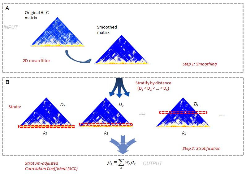
This is a 2-step method (Figure1). In Hi-C data it is often difficult to achieve sufficient coverage. When samples are not sufficiently sequenced, the local variation introduced by under-sampling can make it difficult to capture large domain structures. To reduce local variation, we first smooth the contact map before assessing reproducibility. Although a smoothing filter will reduce the individual spatial resolution, it can improve the contiguity of the regions with elevated interaction, consequently enhancing the domain structures. We use a 2D moving window average filter to smooth the Hi-C contact map. This choice is made for the simplicity and fast computation of mean filter, and the rectangular shape of Hi-C compartments.

In the second step, we stratify the Hi-C reads by the distance of contacting loci, calculate the Pearson correlations within each stratum, and then summarize the stratum-specific correlation coefficients into an aggregated statistic. We name it as Stratum-adjusted Correlation Coefficient (SCC). For the methodology details, please refer to our paper on Genome Research.

knitr::opts_knit$set(progress = TRUE, verbose = TRUE)
library(hicrep)
data("HiCR1")
data("HiCR2")

The format of input and Pre-processing

The input are two Hi-C matrices to be compared. The Hi-C matrices should have the dimension $N\times N$.

dim(HiCR1)
HiCR1[1:10,1:10]

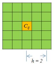
The function get.scc will first smooth the HiC matrix, with given neighborhood size parameter $h$, and filter the bins that have zero counts in both replicates. The arguments includes the two matrices, the resolution of matrices, smoothing parameter, and the lower bound and upper bound of interaction distance considered. The resolution is simply the bin size. Smoothing parameter decides the neighborhood size of smoothing. Below (Figure 2) is a representation of smoothing neighborhood for a point $C_{ij}$:

Calculate Stratum-adjusted Correlation Coefficient (SCC)

An example to calculate SCC for a matrix of 1Mb resolution. Smoothing parameter $h$ is set to 2. The lower bound of distance considered is 0 (diagnal), and the upper bound is 5Mb.

scc.out = get.scc(HiCR1, HiCR2, 1000000, 2, 0, 5000000)

#SCC score
scc.out$scc
#Standard deviation of SCC
scc.out$std

The output is a list of results including stratum specific Pearson correlations, weight coefficient, SCC and the asymptotic standard deviation of SCC. The last two numbers are the ones we needed in most of the situations.

Smooth the Hi-C matrix with 2D mean filter

The function fast.mean.filter() is a very fast algorithm that applies 2D mean filter to squred matrices such as Hi-C contact mapes. The output is a smoothed matrix that has the same size with the original matrix. Here is an example to smooth the matrix with parameter $h = 2$:

smd_mat = fast.mean.filter(HiCR1, 2)

Select the optimal smoothing parameter

To select $h$ objectively, we develop a heuristic procedure to search for the optimal smoothing parameter. Our procedure is designed based on the observation that the correlation between contact maps of replicate samples first increases with the level of smoothness and plateaus when sufficient smoothness is reached.To proceed, we use a pair of reasonably deeply sequenced interaction map as the training data. We randomly sampled 10% of the data, then compute SCC for the sampled dataeach fraction at a series of smoothing parameters in the ascending order. We choose the smallest $h$ at which the increment of the average reproducibility score is less than 0.01. This procedure is repeated ten times, and the mode among the ten $h$’s is picked.

h_hat <- htrain(HiCR1, HiCR2, 1000000, lbr = 0, ubr = 5000000, range = 0:2)

h_hat

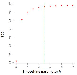
The above graph shows the change of SCC as the $h$ increases from 0 to 10 for a 40Kb resolution matrix. The parameter $h = 5$ is selected as the optimal smoothing neighborhood size.

Important note: The smoothing parameter selection could be confounded by the sequencing depth. Insufficient sequencing depth data might lead to inflated smoothing neighborhood size. To compare SCC between pairs of replicates that has the same resolution, one shall use the same smoothing parameter.

Train the smoothing parameter could be time-consuming. It is not suggested to train $h$ every time when calculating SCC. For a giving resolution, one could use a deeply sequenced biological replicates to train $h$ (i.e., > 300 million total nubmer of reads for whole chromosome), and use the trained $h$ for other same resolution data. Here we provide some trained $h$ trained based on two replicates of hESC cells from Dixon et al 2015 (GEO accession: GSE52457):

Resolution ($h$): 10K (20), 25K (10), 40k(5), 100k(3), 500k(1 or 2), 1M(0 or 1).

Equalize the total number of reads

In previous section, we mention that sequencing depth could be a confounding effect. If the total numbers of reads are very different between the two replicates, it's suggested that one should down-sample the higher sequencing depth to make it equal to the lower one. The best way to do it is to use the bam files to do the sub-sampling randomly. In case you only have the matrix file available, we made a function depth.adj() to do down-sampling from matrix files.

#check total number of reads before adjustment
sum(HiCR1)

# sub-sample 200000 total reads
DS_HiCR1 <- depth.adj(HiCR1, 200000) 

#check total number of reads after adjustment
sum(DS_HiCR1)

sessionInfo()

#check total number of reads before adjustment
sum(HiCR1)

# sub-sample 200000 total reads
DS_HiCR1 <- depth.adj(HiCR1, 200000) 

#check total number of reads after adjustment
sum(DS_HiCR1)

Computation efficiency

Given a pair of contact maps of human chromosome 1 with bin-size equal to 40kb, it takes 27 seconds on a laptop with 2.6GHz Intel Core i7-6600U and 16Gb of RAM.

MonkeyLB/hicrep documentation built on Dec. 15, 2020, 12:47 a.m.