Nothing
README.md
In fgsea: Fast Gene Set Enrichment Analysis


fgsea
An R-package for fast preranked gene set enrichment analysis (GSEA). The package
implements a special algorithm to calculate the empirical enrichment score null distributions simultaneously
for all the gene set sizes, which allows up to several hundred times faster execution time compared to original
Broad implementation. See the preprint for algorithmic details.
Full vignette can be found here: http://bioconductor.org/packages/devel/bioc/vignettes/fgsea/inst/doc/fgsea-tutorial.html
Installation
library(devtools)
install_github("ctlab/fgsea")
Quick run
Loading libraries
library(data.table)
library(fgsea)
library(ggplot2)
Loading example pathways and gene-level statistics:
data(examplePathways)
data(exampleRanks)
Running fgsea (should take about 10 seconds):
fgseaRes <- fgsea(pathways = examplePathways,
                  stats    = exampleRanks,
                  minSize  = 15,
                  maxSize  = 500)
The head of resulting table sorted by p-value:
pathway                                 pval   padj   log2err  ES      NES     size
5990979_Cell_Cycle,_Mitotic             1e-10  4e-09  NA       0.5595  2.7437  317
5990980_Cell_Cycle                      1e-10  4e-09  NA       0.5388  2.6876  369
5990981_DNA_Replication                 1e-10  4e-09  NA       0.6440  2.6390  82
5990987_Synthesis_of_DNA                1e-10  4e-09  NA       0.6479  2.6290  78
5990988_S_Phase                         1e-10  4e-09  NA       0.6013  2.5069  98
5990990_G1_S_Transition                 1e-10  4e-09  NA       0.6233  2.5625  84
5990991_Mitotic_G1-G1_S_phases          1e-10  4e-09  NA       0.6285  2.6256  101
5991209_RHO_GTPase_Effectors            1e-10  4e-09  NA       0.5249  2.3712  157
5991454_M_Phase                         1e-10  4e-09  NA       0.5576  2.5491  173
5991502_Mitotic_Metaphase_and_Anaphase  1e-10  4e-09  NA       0.6053  2.6331  123
As you can see fgsea has a default lower bound eps=1e-10 for estimating P-values. If you need to estimate P-value more accurately, you can set the eps argument to zero in the fgsea function.
fgseaRes <- fgsea(pathways = examplePathways,
                  stats    = exampleRanks,
                  eps      = 0.0,
                  minSize  = 15,
                  maxSize  = 500)

head(fgseaRes[order(pval), ])
pathway                                          pval      padj      log2err  ES      NES     size
5990979_Cell_Cycle,_Mitotic                      4.44e-26  1.70e-23  1.3267   0.5595  2.7414  317
5990980_Cell_Cycle                               5.80e-26  1.70e-23  1.3189   0.5388  2.6747  369
5991851_Mitotic_Prometaphase                     8.50e-19  1.66e-16  1.1239   0.7253  2.9674  82
5992217_Resolution_of_Sister_Chromatid_Cohesion  1.50e-17  2.19e-15  1.0769   0.7348  2.9482  74
5991454_M_Phase                                  1.10e-14  1.29e-12  0.9865   0.5576  2.5436  173
5991599_Separation_of_Sister_Chromatids          3.01e-14  2.94e-12  0.9653   0.6165  2.6630  116
One can make an enrichment plot for a pathway:
plotEnrichment(examplePathways[["5991130_Programmed_Cell_Death"]],
               exampleRanks) + labs(title="Programmed Cell Death")

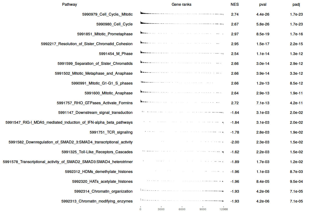
Or make a table plot for a bunch of selected pathways:
topPathwaysUp <- fgseaRes[ES > 0][head(order(pval), n=10), pathway]
topPathwaysDown <- fgseaRes[ES < 0][head(order(pval), n=10), pathway]
topPathways <- c(topPathwaysUp, rev(topPathwaysDown))
plotGseaTable(examplePathways[topPathways], exampleRanks, fgseaRes,
              gseaParam=0.5)
Try the fgsea package in your browser
Any scripts or data that you put into this service are public.
fgsea documentation built on Nov. 8, 2020, 5:22 p.m.
R Package Documentation
Browse R Packages
We want your feedback!
Note that we can't provide technical support on individual packages. You should contact the package authors for that.
![]()
fgsea
An R-package for fast preranked gene set enrichment analysis (GSEA). The package implements a special algorithm to calculate the empirical enrichment score null distributions simultaneously for all the gene set sizes, which allows up to several hundred times faster execution time compared to original Broad implementation. See the preprint for algorithmic details.
Full vignette can be found here: http://bioconductor.org/packages/devel/bioc/vignettes/fgsea/inst/doc/fgsea-tutorial.html
Installation
library(devtools)
install_github("ctlab/fgsea")
Quick run
Loading libraries
library(data.table)
library(fgsea)
library(ggplot2)
Loading example pathways and gene-level statistics:
data(examplePathways)
data(exampleRanks)
Running fgsea (should take about 10 seconds):
fgseaRes <- fgsea(pathways = examplePathways,
stats = exampleRanks,
minSize = 15,
maxSize = 500)
The head of resulting table sorted by p-value:
pathway pval padj log2err ES NES size
5990979_Cell_Cycle,_Mitotic 1e-10 4e-09 NA 0.5595 2.7437 317
5990980_Cell_Cycle 1e-10 4e-09 NA 0.5388 2.6876 369
5990981_DNA_Replication 1e-10 4e-09 NA 0.6440 2.6390 82
5990987_Synthesis_of_DNA 1e-10 4e-09 NA 0.6479 2.6290 78
5990988_S_Phase 1e-10 4e-09 NA 0.6013 2.5069 98
5990990_G1_S_Transition 1e-10 4e-09 NA 0.6233 2.5625 84
5990991_Mitotic_G1-G1_S_phases 1e-10 4e-09 NA 0.6285 2.6256 101
5991209_RHO_GTPase_Effectors 1e-10 4e-09 NA 0.5249 2.3712 157
5991454_M_Phase 1e-10 4e-09 NA 0.5576 2.5491 173
5991502_Mitotic_Metaphase_and_Anaphase 1e-10 4e-09 NA 0.6053 2.6331 123
As you can see fgsea has a default lower bound eps=1e-10 for estimating P-values. If you need to estimate P-value more accurately, you can set the eps argument to zero in the fgsea function.
fgseaRes <- fgsea(pathways = examplePathways,
stats = exampleRanks,
eps = 0.0,
minSize = 15,
maxSize = 500)
head(fgseaRes[order(pval), ])
pathway pval padj log2err ES NES size
5990979_Cell_Cycle,_Mitotic 4.44e-26 1.70e-23 1.3267 0.5595 2.7414 317
5990980_Cell_Cycle 5.80e-26 1.70e-23 1.3189 0.5388 2.6747 369
5991851_Mitotic_Prometaphase 8.50e-19 1.66e-16 1.1239 0.7253 2.9674 82
5992217_Resolution_of_Sister_Chromatid_Cohesion 1.50e-17 2.19e-15 1.0769 0.7348 2.9482 74
5991454_M_Phase 1.10e-14 1.29e-12 0.9865 0.5576 2.5436 173
5991599_Separation_of_Sister_Chromatids 3.01e-14 2.94e-12 0.9653 0.6165 2.6630 116
One can make an enrichment plot for a pathway:
plotEnrichment(examplePathways[["5991130_Programmed_Cell_Death"]],
exampleRanks) + labs(title="Programmed Cell Death")
Or make a table plot for a bunch of selected pathways:
topPathwaysUp <- fgseaRes[ES > 0][head(order(pval), n=10), pathway]
topPathwaysDown <- fgseaRes[ES < 0][head(order(pval), n=10), pathway]
topPathways <- c(topPathwaysUp, rev(topPathwaysDown))
plotGseaTable(examplePathways[topPathways], exampleRanks, fgseaRes,
gseaParam=0.5)
Try the fgsea package in your browser
Any scripts or data that you put into this service are public.
R Package Documentation
Browse R Packages
We want your feedback!
Note that we can't provide technical support on individual packages. You should contact the package authors for that.
Embedding an R snippet on your website
Add the following code to your website.
For more information on customizing the embed code, read Embedding Snippets.