README.md

In js2264/cooleR: Analysing cool files in R with HiContacts

HiContacts

👉 OHCA book 📖

HiContacts provides tools to investigate (m)cool matrices imported in R by HiCExperiment.

It leverages the HiCExperiment class of objects, built on pre-existing Bioconductor objects, namely InteractionSet, GInterations and ContactMatrix (Lun, Perry & Ing-Simmons, F1000Research 2016), and provides analytical and visualization tools to investigate contact maps.

Installation

HiContacts is available in Bioconductor. To install the current release, use:

if (!requireNamespace("BiocManager", quietly = TRUE))
    install.packages("BiocManager")
BiocManager::install("HiContacts")

To install the most recent version of HiContacts, you can use:

install.packages("devtools")
devtools::install_github("js2264/HiContacts")
library(HiContacts)

Citation

If you are using HiContacts in your research, please cite:

Serizay J (2022). HiContacts: HiContacts: R interface to cool files. R package version 1.1.0 https://github.com/js2264/HiContacts.

How to use HiContacts

HiContacts includes a introduction vignette where its usage is illustrated. To access the vignette, please use:

vignette('HiContacts')

Visualising Hi-C contact maps and features

Importing a Hi-C contact maps file with HiCExperiment

mcool_file <- HiContactsData::HiContactsData('yeast_wt', format = 'mcool')
range <- 'I:20000-80000' # range of interest
availableResolutions(mcool_file)
hic <- HiCExperiment::import(mcool_file, format = 'mcool', focus = range, resolution = 1000)
hic

Plotting matrices (square or horizontal)

plotMatrix(hic, use.scores = 'count')
plotMatrix(hic, use.scores = 'balanced', limits = c(-4, -1))
plotMatrix(hic, use.scores = 'balanced', limits = c(-4, -1), maxDistance = 100000)

Plotting matrices with topological features

library(rtracklayer)
mcool_file <- HiContactsData::HiContactsData('yeast_wt', format = 'mcool')
hic <- import(mcool_file, format = 'mcool', focus = 'IV')
loops <- system.file("extdata", 'S288C-loops.bedpe', package = 'HiContacts') |> 
    import() |> 
    InteractionSet::makeGInteractionsFromGRangesPairs()
borders <- system.file("extdata", 'S288C-borders.bed', package = 'HiContacts') |> 
    import()
p <- plotMatrix(
    hic, loops = loops, borders = borders, 
    limits = c(-4, -1), dpi = 120
)

Plotting aggregated matrices (a.k.a. APA plots)

contacts <- contacts_yeast()
contacts <- zoom(contacts, resolution = 2000)
aggr_centros <- aggregate(contacts, targets = topologicalFeatures(contacts, 'centromeres'))
plotMatrix(aggr_centros, use.scores = 'detrended', limits = c(-1, 1), scale = 'linear')

Mapping topological features

Chromosome compartments

microC_mcool <- fourDNData::fourDNData('4DNES14CNC1I', 'mcool')
hic <- import(microC_mcool, format = 'mcool', resolution = 10000000)
genome <- BSgenome.Mmusculus.UCSC.mm10::BSgenome.Mmusculus.UCSC.mm10

# - Get compartments
hic <- getCompartments(
    hic, resolution = 100000, genome = genome, chromosomes = c('chr17', 'chr19')
)

# - Export compartments as bigwig and bed files
export(IRanges::coverage(metadata(hic)$eigens, weight = 'eigen'), 'microC_compartments.bw')
export(
    topologicalFeatures(hic, 'compartments')[topologicalFeatures(hic, 'compartments')$compartment == 'A'], 
    'microC_A-compartments.bed'
)
export(
    topologicalFeatures(hic, 'compartments')[topologicalFeatures(hic, 'compartments')$compartment == 'B'], 
    'microC_B-compartments.bed'
)

# - Generate saddle plot
plotSaddle(hic)

Diamond insulation score and chromatin domains borders

# - Compute insulation score
hic <- refocus(hic, 'chr19:1-30000000') |> 
    zoom(resolution = 10000) |> 
    getDiamondInsulation(window_size = 100000) |> 
    getBorders()

# - Export insulation as bigwig track and borders as bed file
export(IRanges::coverage(metadata(hic)$insulation, weight = 'insulation'), 'microC_insulation.bw')
export(topologicalFeatures(hic, 'borders'), 'microC_borders.bed')

In-depth analysis of HiCExperiment objects

Arithmetics

Detrend

Autocorrelate

Divide

Merge

Distance law, a.k.a. P(s)

hic <- import(CoolFile(
    mcool_file, 
    pairs = HiContactsData::HiContactsData('yeast_wt', format = 'pairs.gz')
))
ps <- distanceLaw(hic)
plotPs(ps, ggplot2::aes(x = binned_distance, y = norm_p))

Virtual 4C

hic <- import(CoolFile(mcool_file))
v4C <- virtual4C(hic, viewpoint = GRanges('V:150000-170000'))
plot4C(v4C)

Cis-trans ratios

hic <- import(CoolFile(mcool_file))
cisTransRatio(hic)

Scalograms

HiCExperiment ecosystem

HiCool is integrated within the HiCExperiment ecosystem in Bioconductor. Read more about the HiCExperiment class and handling Hi-C data in R here.

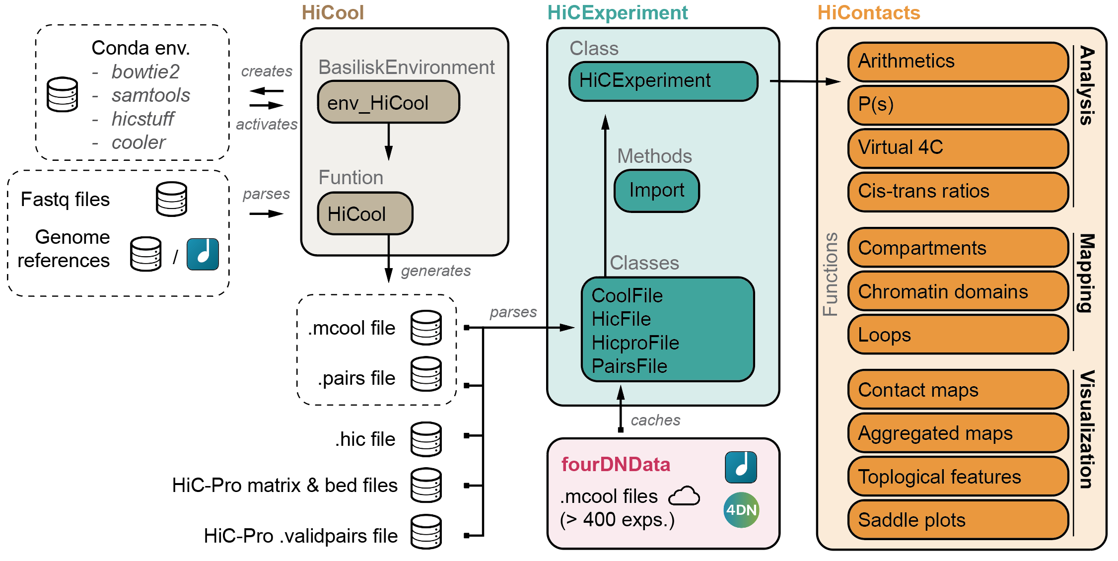
• HiCExperiment: Parsing Hi-C files in R
• HiCool: End-to-end integrated workflow to process fastq files into .cool and .pairs files
• HiContacts: Investigating Hi-C results in R
• HiContactsData: Data companion package
• fourDNData: Gateway package to 4DN-hosted Hi-C experiments

js2264/cooleR documentation built on Jan. 29, 2024, 10:47 p.m.