In saezlab/decoupleR: decoupleR: Ensemble of computational methods to infer biological activities from omics data

knitr::opts_chunk$set(
    collapse = TRUE,
    comment = "#>"
)

Bulk RNA-seq yield many molecular readouts that are hard to interpret by themselves. One way of summarizing this information is by inferring pathway activities from prior knowledge.

In this notebook we showcase how to use decoupleR for pathway activity inference with a bulk RNA-seq data-set where the transcription factor FOXA2 was knocked out in pancreatic cancer cell lines.

The data consists of 3 Wild Type (WT) samples and 3 Knock Outs (KO). They are freely available in GEO.

Loading packages

First, we need to load the relevant packages:

## We load the required packages
library(decoupleR)
library(dplyr)
library(tibble)
library(tidyr)
library(ggplot2)
library(pheatmap)
library(ggrepel)

Loading the data-set

Here we used an already processed bulk RNA-seq data-set. We provide the normalized log-transformed counts, the experimental design meta-data and the Differential Expressed Genes (DEGs) obtained using limma.

For this example we use limma but we could have used DeSeq2, edgeR or any other statistical framework. decoupleR requires a gene level statistic to perform enrichment analysis but it is agnostic of how it was generated. However, we do recommend to use statistics that include the direction of change and its significance, for example the t-value obtained for limma(t) or DeSeq2(stat). edgeR does not return such statistic but we can create our own by weighting the obtained logFC by pvalue with this formula: -log10(pvalue) * logFC.

We can open the data like this:

inputs_dir <- system.file("extdata", package = "decoupleR")
data <- readRDS(file.path(inputs_dir, "bk_data.rds"))

From data we can extract the mentioned information. Here we see the normalized log-transformed counts:

# Remove NAs and set row names
counts <- data$counts %>%
  dplyr::mutate_if(~ any(is.na(.x)), ~ if_else(is.na(.x),0,.x)) %>% 
  column_to_rownames(var = "gene") %>% 
  as.matrix()
head(counts)

The design meta-data:

design <- data$design
design

And the results of limma, of which we are interested in extracting the obtained t-value from the contrast:

# Extract t-values per gene
deg <- data$limma_ttop %>%
    select(ID, t) %>% 
    filter(!is.na(t)) %>% 
    column_to_rownames(var = "ID") %>%
    as.matrix()
head(deg)

PROGENy model

PROGENy is a comprehensive resource containing a curated collection of pathways and their target genes, with weights for each interaction. For this example we will use the human weights (other organisms are available) and we will use the top 500 responsive genes ranked by p-value. Here is a brief description of each pathway:

• Androgen: involved in the growth and development of the male reproductive organs.
• EGFR: regulates growth, survival, migration, apoptosis, proliferation, and differentiation in mammalian cells
• Estrogen: promotes the growth and development of the female reproductive organs.
• Hypoxia: promotes angiogenesis and metabolic reprogramming when O2 levels are low.
• JAK-STAT: involved in immunity, cell division, cell death, and tumor formation.
• MAPK: integrates external signals and promotes cell growth and proliferation.
• NFkB: regulates immune response, cytokine production and cell survival.
• p53: regulates cell cycle, apoptosis, DNA repair and tumor suppression.
• PI3K: promotes growth and proliferation.
• TGFb: involved in development, homeostasis, and repair of most tissues.
• TNFa: mediates haematopoiesis, immune surveillance, tumour regression and protection from infection.
• Trail: induces apoptosis.
• VEGF: mediates angiogenesis, vascular permeability, and cell migration.
• WNT: regulates organ morphogenesis during development and tissue repair.

To access it we can use decoupleR:

net <- get_progeny(organism = 'human', top = 500)
net

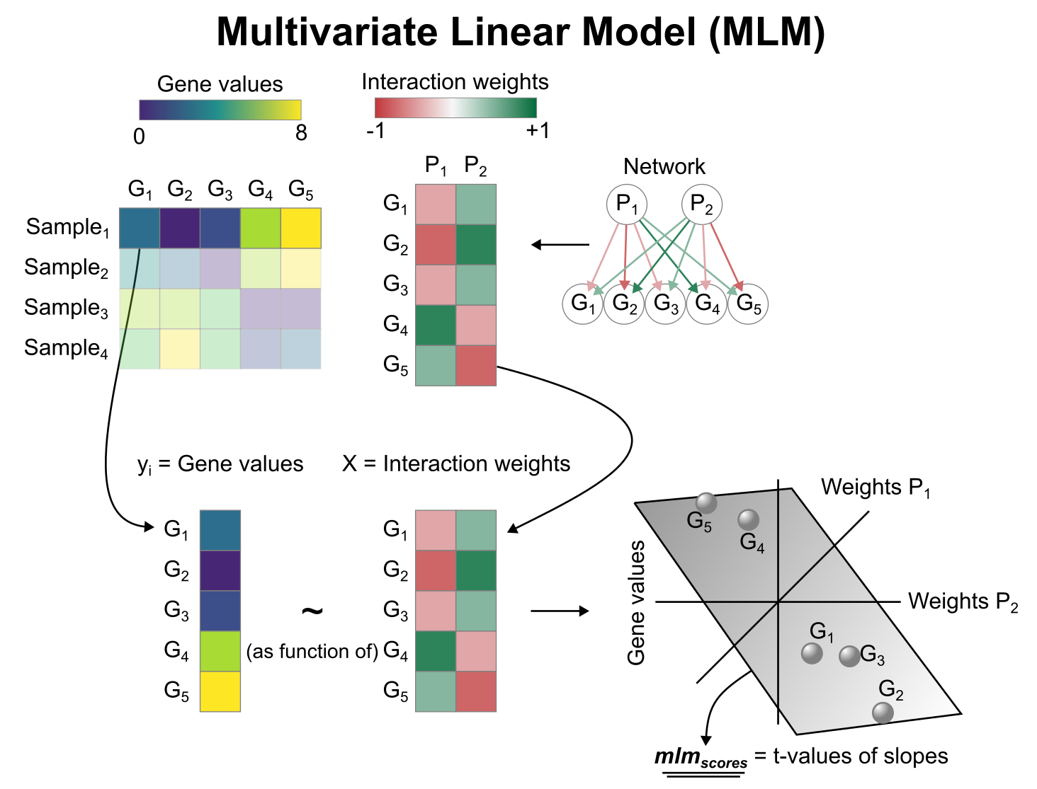
Activity inference with Multivariate Linear Model (MLM)

To infer pathway enrichment scores we will run the Multivariate Linear Model (mlm) method. For each sample in our dataset (mat), it fits a linear model that predicts the observed gene expression based on all pathways' Pathway-Gene interactions weights. Once fitted, the obtained t-values of the slopes are the scores. If it is positive, we interpret that the pathway is active and if it is negative we interpret that it is inactive.

To run decoupleR methods, we need an input matrix (mat), an input prior knowledge network/resource (net), and the name of the columns of net that we want to use.

# Run mlm
sample_acts <- run_mlm(mat=counts, net=net, .source='source', .target='target',
                  .mor='weight', minsize = 5)
sample_acts

Visualization

From the obtained results we will observe the obtained activities per sample in a heat-map:

# Transform to wide matrix
sample_acts_mat <- sample_acts %>%
  pivot_wider(id_cols = 'condition', names_from = 'source',
              values_from = 'score') %>%
  column_to_rownames('condition') %>%
  as.matrix()

# Scale per feature
sample_acts_mat <- scale(sample_acts_mat)

# Choose color palette
palette_length = 100
my_color = colorRampPalette(c("Darkblue", "white","red"))(palette_length)

my_breaks <- c(seq(-3, 0, length.out=ceiling(palette_length/2) + 1),
               seq(0.05, 3, length.out=floor(palette_length/2)))

# Plot
pheatmap(sample_acts_mat, border_color = NA, color=my_color, breaks = my_breaks) 

We can also infer pathway activities from the t-values of the DEGs between KO and WT:

# Run mlm
contrast_acts <- run_mlm(mat=deg, net=net, .source='source', .target='target',
                  .mor='weight', minsize = 5)
contrast_acts

Let's show the changes in activity between KO and WT:

# Plot
ggplot(contrast_acts, aes(x = reorder(source, score), y = score)) + 
    geom_bar(aes(fill = score), stat = "identity") +
    scale_fill_gradient2(low = "darkblue", high = "indianred", 
        mid = "whitesmoke", midpoint = 0) + 
    theme_minimal() +
    theme(axis.title = element_text(face = "bold", size = 12),
        axis.text.x = 
            element_text(angle = 45, hjust = 1, size =10, face= "bold"),
        axis.text.y = element_text(size =10, face= "bold"),
        panel.grid.major = element_blank(), 
        panel.grid.minor = element_blank()) +
    xlab("Pathways")

The pathway p53 and Trail are deactivated in KO when compared to WT, while MAPKK and JAK-STAT and seem to be activated.

We can further visualize the most responsive genes in each pathway along their t-values to interpret the results. For example, let's see the genes that are belong to the MAPK pathway:

pathway <- 'MAPK'

df <- net %>%
  filter(source == pathway) %>%
  arrange(target) %>%
  mutate(ID = target, color = "3") %>%
  column_to_rownames('target')
inter <- sort(intersect(rownames(deg),rownames(df)))
df <- df[inter, ]
df['t_value'] <- deg[inter, ]
df <- df %>%
  mutate(color = if_else(weight > 0 & t_value > 0, '1', color)) %>%
  mutate(color = if_else(weight > 0 & t_value < 0, '2', color)) %>%
  mutate(color = if_else(weight < 0 & t_value > 0, '2', color)) %>%
  mutate(color = if_else(weight < 0 & t_value < 0, '1', color))

ggplot(df, aes(x = weight, y = t_value, color = color)) + geom_point() +
  scale_colour_manual(values = c("red","royalblue3","grey")) +
  geom_label_repel(aes(label = ID)) + 
  theme_minimal() +
  theme(legend.position = "none") +
  geom_vline(xintercept = 0, linetype = 'dotted') +
  geom_hline(yintercept = 0, linetype = 'dotted') +
  ggtitle(pathway)

The pathway seems to be active since the majority of target genes with positive weights have positive t-values (1st quadrant), and the majority of the ones with negative weights have negative t-values (3d quadrant).

Session information

options(width = 120)
sessioninfo::session_info()

saezlab/decoupleR documentation built on April 12, 2024, 10:41 a.m.