README.md

In microresearcher/MicroVis: Microbiome Analysis and Visualization

MicroVis

MicroVis is a package for flexible analysis of metagenomic data and generation of customizable, publication-ready figures. This version was built under R 4.0.1

Examples

The following analysis and figures are examples of what MicroVis can do. These results have been generated using a 2012 study by Kostic et al (linked in the walk-through below) examining the gut microbiome of human colorectal cancer versus healthy controls. The walk-through below (not yet complete) will guide you through the steps to do this analysis and make these figures with the same data.

Alpha Diversity

Beta Diversity (unweighted unifrac)

Statistics shown in the figure are calculated from a PERMANOVA analysis using the "adonis" function from the vegan package

Stacked Abundance Barplots

Random Forest Feature Selection

These features are selected by training a random forest model, then using the Boruta algorithm to identify features with a statistically significant impact on predicting Healthy vs Tumor.

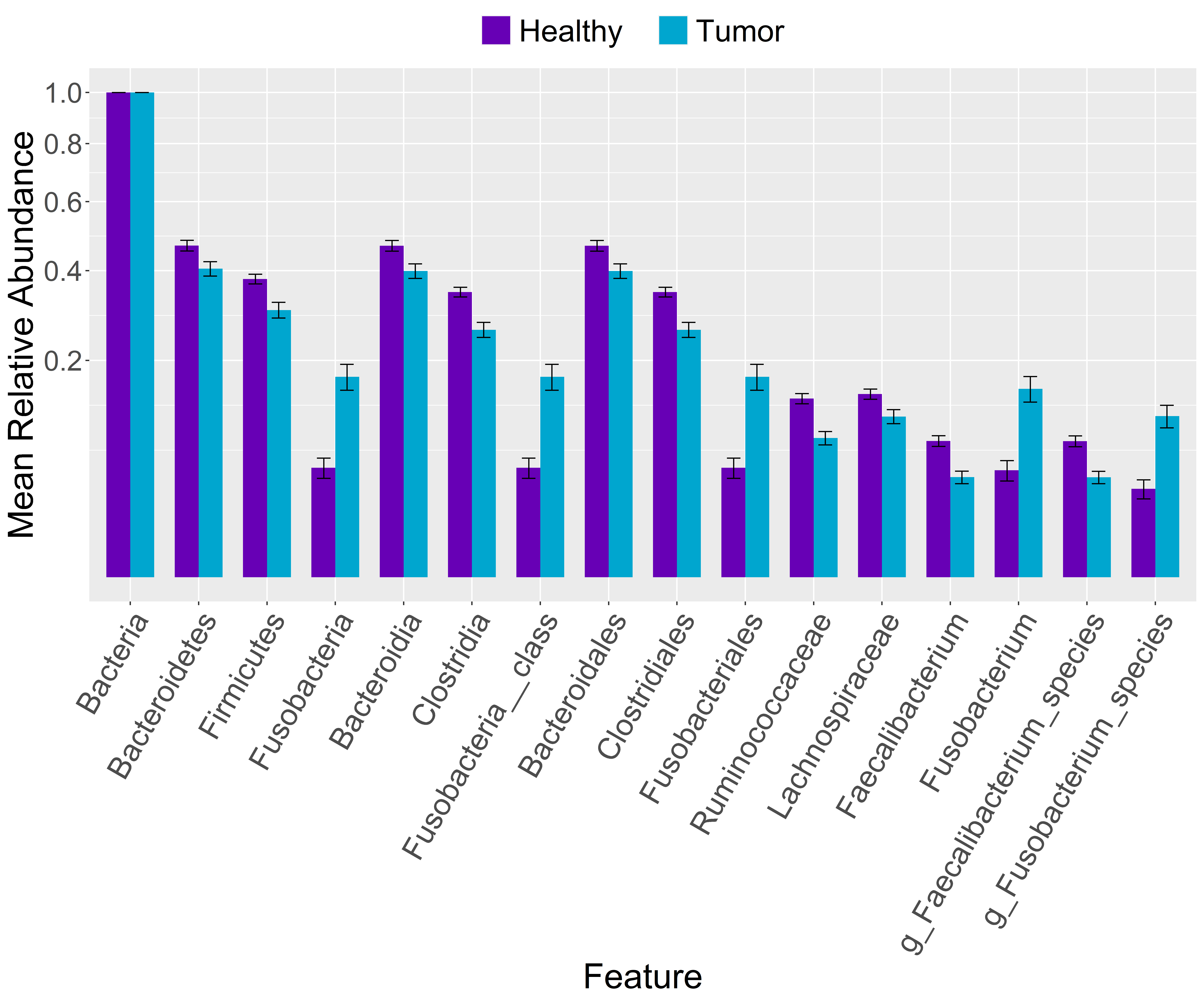
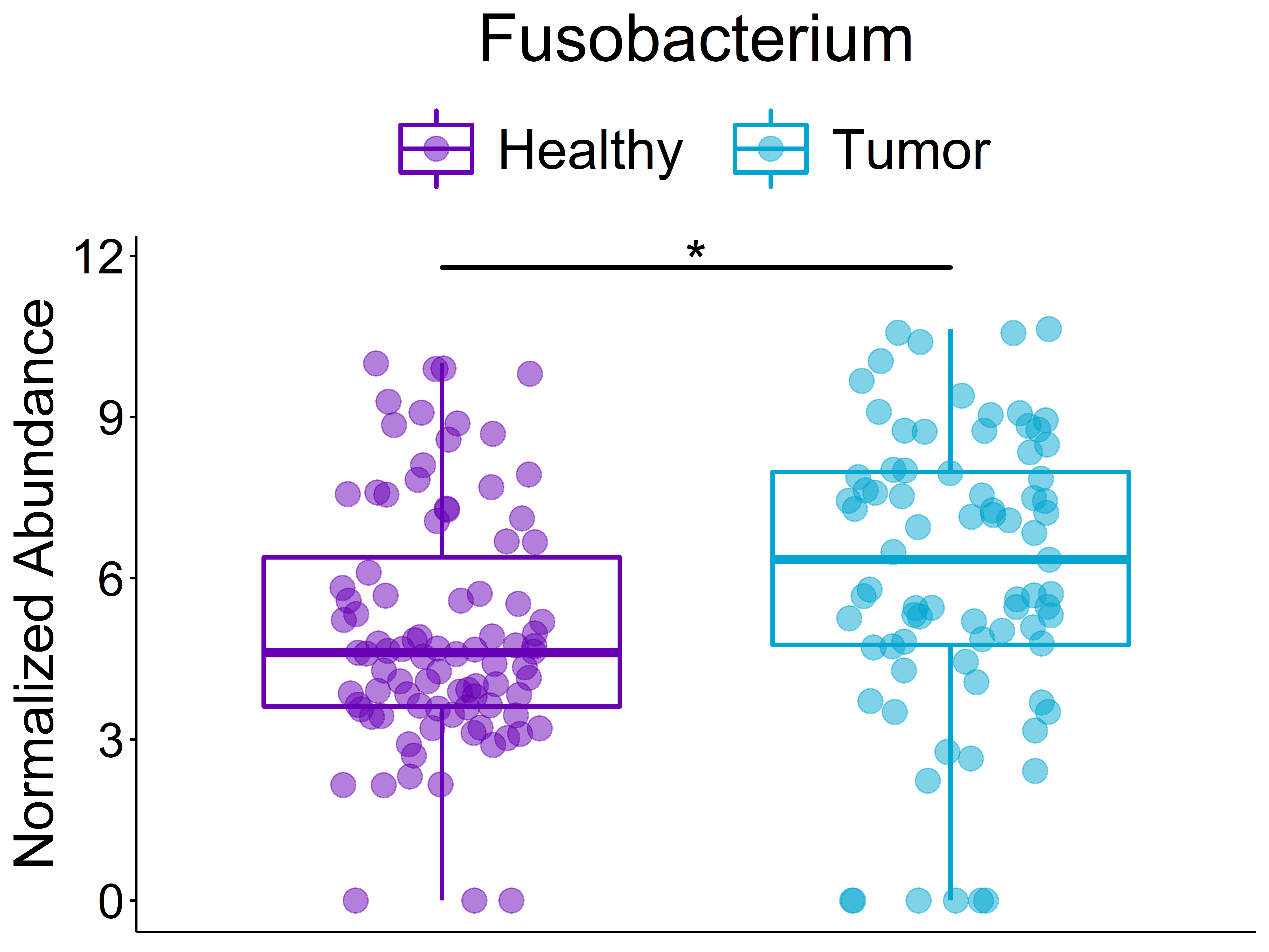
Classic Univariate Analysis

These are done using Wilcoxon rank sum tests and then corrected for multiple comparisons using the Benjamini-Hochberg method.

Bar graph of significantly different features at the phylum to genus ranks

Boxplot of Fusobacterium genus

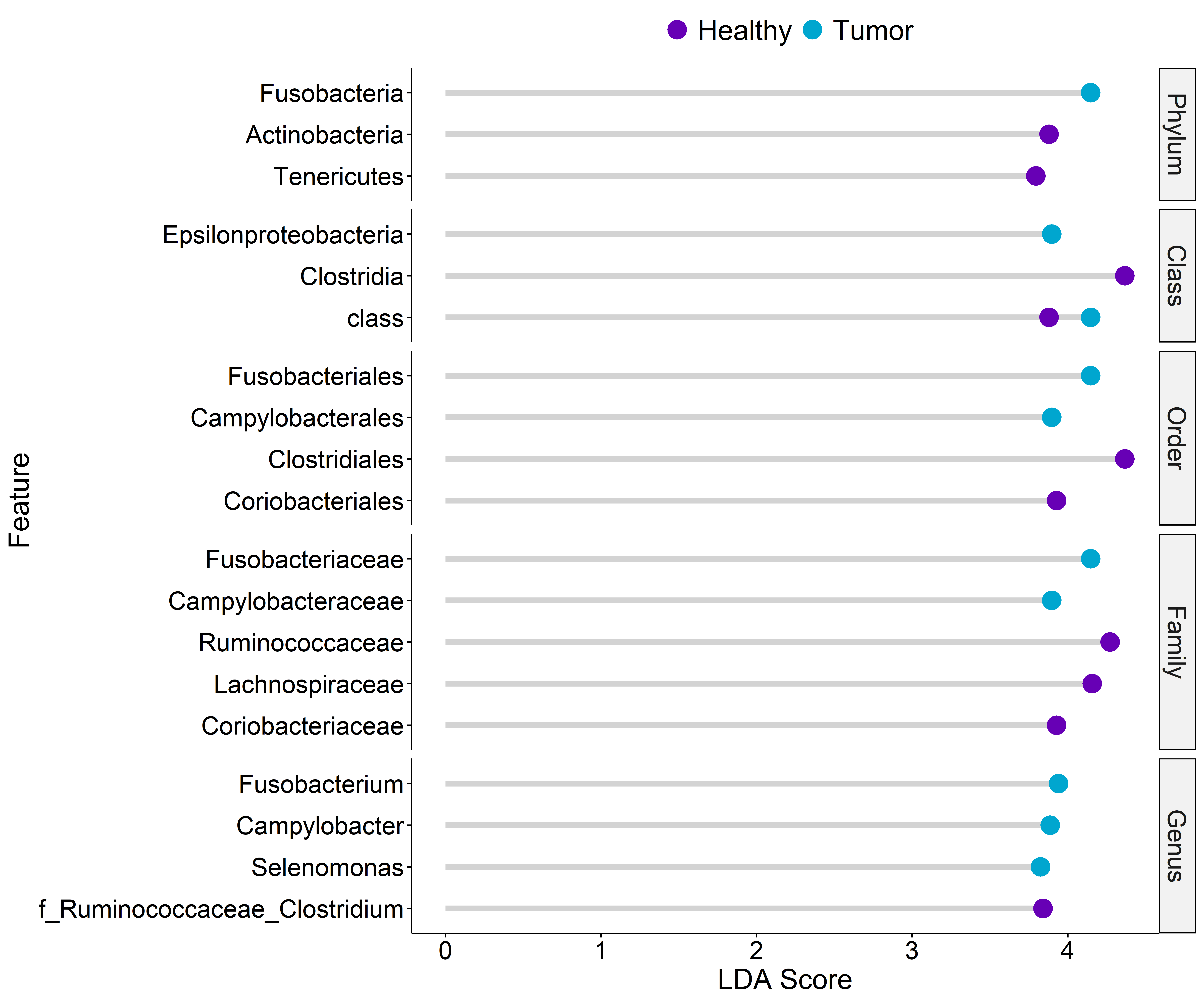
Linear discriminant analysis Effect Size (LEfSe)

Installation

Before installing MicroVis, make sure to install these dependencies separately for full functionality:

Install phyloseq, DESeq2, and ComplexHeatmap with BiocManager:

if (!requireNamespace("BiocManager", quietly = TRUE)) install.packages("BiocManager")

BiocManager::install("phyloseq")
BiocManager::install("DESeq2")
BiocManager::install("ComplexHeatmap")

Install microbiomemarker from GitHub with devtools:

if (!require("devtools")) install.packages("devtools")

devtools::install_github("yiluheihei/microbiomeMarker") 

You can then install the latest version of MicroVis from GitHub:

devtools::install_github("https://github.com/microresearcher/MicroVis.git")

Example

The following steps will walk you through some of the basic analysis and plotting functions that MicroVis offers. We will be using publicly available data from:

Genomic analysis identifies association of Fusobacterium with colorectal carcinoma. Kostic, A. D., Gevers, D., Pedamallu, C. S., Michaud, M., Duke, F., Earl, A. M., et al. (2012). Genome research, 22(2), 292-298.

This example data comes with this package, it just needs to be loaded in. First, load up MicroVis:

library(MicroVis)

Loading Data

Now let's grab the example data

kostic_files <- system.file('extdata',package='MicroVis')
mvload(kostic_files)

A pop-up window will appear showing the files in kostic_files and asking you to select the metadata file. Double click kostic2012_metadata_short.csv in the pop-up window to select it. Next, it will ask if you would like to load a taxonomic dataset. Enter 1 for "Yes" in the RStudio console. It will then ask you to select the taxonomy abundance file. Double click kostic2012_taxonomy_abundance.csv and the data will start loading.

• As the data loads, MicroVis will ask you a few questions about the data. The first question will ask what the factors (independent variables) are in this dataset. For now, just select "DIAGNOSIS"
• It will then show you the groups in the factor you selected, and ask if you would like to change the order. We will keep the current order for now, so enter 1
• Next, it will show you the read depths for all the samples in the abundance file and ask if you would like to change the read count threshold. Enter 2 to change the threshold and then enter 1000 as a new threshold
  • This threshold is used to determine what samples were likely poorly/insufficiently sequenced and thus not valuable for data analysis. In this dataset (remember this is from 2012!), we can see that most of the samples fall below our default threshold of 10,000 reads per sample

MicroVis will then go ahead and automatically process the data with normalization and filtering steps. It then creates two datasets, a taxa_raw with the pre-processed data and a taxa_proc with the automatically processed data. You can undo any of these processing steps and apply different ones if you want, which will be covered in a later example.

Selecting Groups to Analyze

You might notice that the "None" group only has four samples. Additionally, we are interested in comparing healthy versus tumor samples, and we don't know what the "None" group corresponds to, so we will remove that group with the removeGrps() function

removeGrps()

It will then ask you to select one or more groups to remove. Enter 2 or select the "None" group in the pop-up if one shows up and hit "Ok". After this, the data will be re-processed without these 4 samples.

Analyzing and Making Figures

The taxa_proc dataset is loaded up as the active dataset (active_dataset), meaning you do not need to type out its name when running the analysis or plotting functions.

First, let us look at the overall bacterial richness of the three groups, "Healthy", "None", and "Tumor", by plotting their Chao1 alpha diversities

plotAlphaDiv()

microresearcher/MicroVis documentation built on Feb. 8, 2024, 10:59 a.m.