In wguo-research/scCancer: A package for automated processing of single cell RNA-seq data in cancer

  BiocStyle::markdown()

knitr::opts_chunk$set(
  collapse = TRUE,
  comment = "#>"
)

Introduction

Molecular heterogeneities bring great challenges for cancer diagnosis and treatment. Recent advances in single cell RNA-sequencing (scRNA-seq) technology make it possible to study cancer transcriptomic heterogeneities at single cell level.

Here, we develop an R package named scCancer which focuses on processing and analyzing scRNA-seq data for cancer research. Except basic data processing steps, this package takes several special considerations for cancer-specific features.

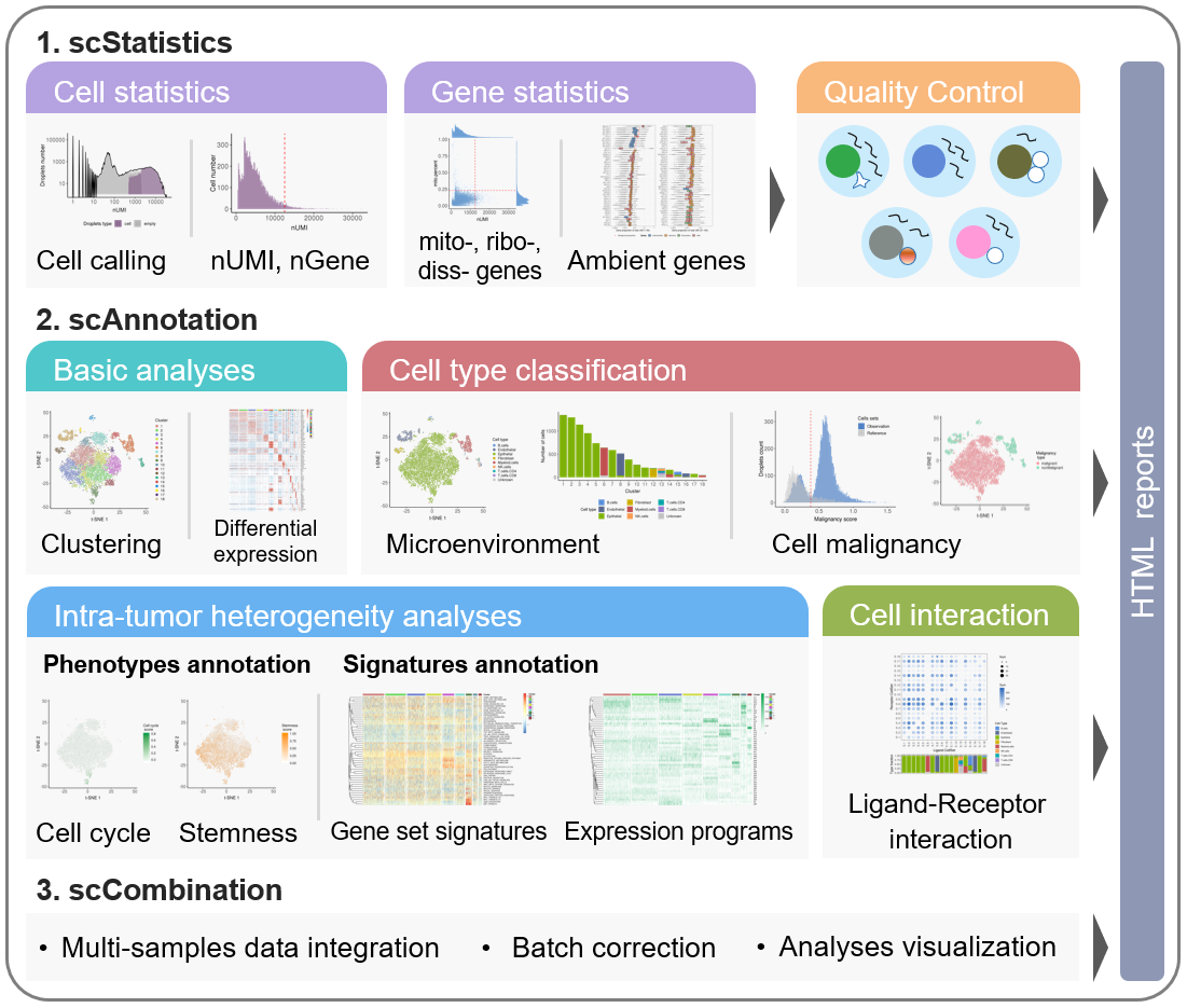
The workflow of scCancer mainly consists of three modules: scStatistics, scAnnotation, and scCombination.

• The scStatistics performs basic statistical analyses of raw data and quality control.

• The scAnnotation performs functional data analyses and visualizations, such as low dimensional representation, clustering, cell type classification, cell malignancy estimation, cellular phenotype analyses, gene signature analyses, cell-cell interaction analyses, etc.

• The scCombination perform multiple samples data integration, batch effect correction and analyses visualization.

After the computational analyses, detailed and graphical reports were generated in user-friendly HTML format.

Basic instructions

System Requirements

• R version: >= 3.5.0

Installation

Firstly, please install or update the package devtools by running

install.packages("devtools")

Then the scCancer can be installed via

library(devtools)
devtools::install_github("wguo-research/scCancer")

Hint:

1) A dependent package NNLM was removed from the CRAN repository recently, so an error about it may be reported during the installation. If so, you can install a formerly available version manually from its archive.

2) Some dependent packages on GitHub (as follows) may not be able to install automatically, if you encounter such errors, please refer to their GitHub and install them via corresponding commands. * SoupX: * Link: GitHub * Installation: devtools::install_github("constantAmateur/SoupX")

• harmony:

  • Link: GitHub
  • Installation: devtools::install_github("immunogenomics/harmony")

• liger:

  • Link: GitHub
  • Installation: devtools::install_github("MacoskoLab/liger")

Loading

library(scCancer)

Data preparation

The scCancer is mainly designed for 10X Genomics platform, and it requires a data folder containing the results generated by the software Cell Ranger. In general, the data folder needs to be organized as following which is the output of Cell Ranger V3:

    /sampleFolder
    ├── filtered_feature_bc_matrix
    │   ├── barcodes.tsv.gz
    │   ├── features.tsv.gz
    │   └── matrix.mtx.gz
    ├── raw_feature_bc_matrix
    │   ├── barcodes.tsv.gz
    │   ├── features.tsv.gz
    │   └── matrix.mtx.gz
    └── web_summary.html

Comparing to Cell Ranger V2 (CR2), Cell Ranger V3 (CR3) can identify cells with low RNA content better. So we suggest to use CR3 to do alignment and cell-calling. Considering that some published data is from CR2 or the raw matrix isn't supported, we specially deisgn the pipeline to be compatible with these situations. A common folder structure of CR2 is as below.

    /sampleFolder
    ├── filtered_gene_bc_matrices
    │   └── hg19
    │       ├── barcodes.tsv
    │       ├── genes.tsv
    │       └── matrix.mtx
    ├── raw_gene_bc_matrices
    │   └── hg19
    │       ├── barcodes.tsv
    │       ├── genes.tsv
    │       └── matrix.mtx
    └── web_summary.html

For other droplet-based platforms, the data folder should be prepared likewise.

Quick start

Here, we provide an example data of kidney cancer from 10X Genomics. Users can download it and run following scripts to understand the workflow of scCancer. And following are the generated HTML reports:

• report-scStat.html
• report-scAnno.html

For multi-samples, following is a generated HTML report for three kidney cancer samples integration analysis:

• report-scAnnoComb.html

scStatistics

The scStatistics mainly implements quality control for the expression matrix and returns some suggested thresholds to filter cells and genes. Meanwhile, to evaluate the influence of ambient RNAs from lysed cells better, this step also estimates the contamination fraction by using the algorithm of SoupX.

Following is the example script to run the first module scStatistics. And using help(runScStatistics) can get more details about its arguments to realize personalized setting.

library(scCancer)

# A path containing the cell ranger processed data
dataPath <- "./data/KC-example"
# A path used to save the results files
savePath <- "./results/KC-example"
# The sample name
sampleName <- "KC-example"
# The author name or a string used to mark the report.
authorName <- "G-Lab@THU"

# Run scStatistics
stat.results <- runScStatistics(
    dataPath = dataPath,
    savePath = savePath,
    sampleName = sampleName,
    authorName = authorName
)

Running the scStatistics script will generate some files/folders as below:

1. report-scStat.html : A HTML report containing all results.
2. report-scStat.md : A markdown report.
3. figures\/ : All figures generated during this module.
4. report-figures\/ : All figures presented in the HTML report.
5. cellManifest-all.txt : The statistical results for all droplets.
6. cell.QC.thres.txt : The suggested thresholds to filter poor-quality cells.
7. geneManifest.txt : The statistical results for genes.
8. ambientRNA-SoupX.txt : The results of estimating contamination fraction.
9. report-cellRanger.html : The summary report generated by Cell Ranger.

scAnnotation

Using the QC thresholds, the scAnnotation filters cells and genes firstly, and then performs basic operations (normalization, log-transformation, highly variable genes identification, unwanted variance removing, scaling, centering, dimension reduction, clustering, and differential expression analysis) using R package Seurat V3. Besides, scAnnotation also performs some cancer-specific analyses:

• Doublet score estimation : In this step, we integrate two methods (binary classification based bcds and co-expression based cxds) of R package scds to estimate doublet scores.

• Cancer micro-environmental cell type classification : In this step, we develop a data-driven OCLR (one-class logistic regression) model to predict cell types, including epithelial cells, endothelial cells, fibroblasts, and immune cells (CD4+ T cells, CD8+ T cells, B cells, nature killer cells, and myeloid cells).

• Cell malignancy estimation : In this step, we refer to the algorithm of R package infercnv to estimate an initial CNV profiles. Then, we take advantage of cells’ neighbor information to smooth CNV values and define the malignancy score as the mean of the squares of them.

• Cell cycle analysis : In this step, to analyze intra-tumor cell phenotype heterogeneity, we define cell cycle score as the relative average expression of a list of G2/M and S phase markers, by using the function “AddModuleScore” of Seurat.

• Cell stemness analysis : In this step, to analyze intra-tumor cell phenotype heterogeneity, we define cell stemness score as the Spearman correlation coefficient between cells’ expression and our pre-trained stemness signature, by referring to the algorithm of Malta et al.

• Gene set signature analysis : In this step, to analyze intra-tumor heterogeneity at gene sets level, we provide two methods to calculated gene set signature scores: GSVA and relative average expression levels. By default, we use 50 hallmark gene sets from MSigDB.

• Expression programs identification : In this step, to analyze intra-tumor heterogeneity at gene sets level, we use non-negative matrix factorization (NMF) to unsupervisedly identify potential expression program signatures.

• Cell-cell interaction analyses : In this step, we referred to the methods of Kumar et al to characterize ligand-receptor interactions across cell clusters.

Following is the example script to run the second module scAnnotation. And using help(runScAnnotation) can get more details about its arguments to realize personalized setting.

library(scCancer)

# A path containing the cell ranger processed data
dataPath <- "./data/KC-example"    
# A path containing the scStatistics results
statPath <- "./results/KC-example" 
# A path used to save the results files
savePath <- "./results/KC-example" 
# The sample name
sampleName <- "KC-example"
# The author name or a string used to mark the report.
authorName <- "G-Lab@THU"    

# Run scAnnotation
anno.results <- runScAnnotation(
    dataPath = dataPath,
    statPath = statPath,
    savePath = savePath,
    authorName = authorName,
    sampleName = sampleName,
    geneSet.method = "average"   # or "GSVA"
)

Running the scAnnotation script will generate some files/folders as below:

1. report-scAnno.html : A HTML report containing all results.
2. report-scAnno.md : A markdown report.
3. figures\/ : All figures generated during this module.
4. report-figures\/ : All figures presented in the HTML report.
5. geneManifest.txt : The annotation results of genes updated by filter information.
6. expr.RDS : A Seurat object.
7. diff.expr.genes\/ : Differentially expressed genes information for all clusters.
8. cellAnnotation.txt : The annotation results for each cells.
9. malignancy\/: All results of cell malignancy estimation.
10. expr.programs\/ : All results of expression programs identification.
11. InteractionScore.txt : Cell clusters interactions scores.

scCombination

The scCombination mainly performs multiple samples data integration, batch effect correction and analyses visualization based on the scAnnotation results of single sample. And four strategies (NormalMNN (default), SeuratMNN, Raw and Regression) to integrate data and correct batch effect are optional.

Following is the example script to run the module scCombination. And using help(runScCombination) can get more details about its arguments.

library(scCancer)

# Paths containing the results of 'runScAnnotation' for each sample.
single.savePaths <- c("./results/KC1", "./results/KC2", "./results/KC3")
# Labels for all samples.
sampleNames <- c("KC1", "KC2", "KC3")
# A path used to save the results files
savePath <- "./results/KC123-comb"
# A label for the combined samples.
combName <- "KC123-comb"
# The author name or a string used to mark the report.
authorName <- "G-Lab@THU"
# The method to combine data.
comb.method <- "NormalMNN"  # SeuratMNN  Raw  Regression

# Run scCombination
comb.results <- runScCombination(
    single.savePaths = single.savePaths, 
    sampleNames = sampleNames, 
    savePath = savePath, 
    combName = combName,
    authorName = authorName,
    comb.method = comb.method
)    

Running the scAnnotation script will generate some files/folders as below:

1. report-scAnnoComb.html : A HTML report containing all results.
2. report-scAnnoComb.md : A markdown report.
3. figures\/ : All figures generated during this step.
4. report-figures\/ : All figures presented in the HTML report.
5. expr.RDS : A Seurat object.
6. diff.expr.genes\/ : Differentially expressed genes information for all clusters.
7. cellAnnotation.txt : The annotation results for each cells.
8. expr.programs\/ : All results of expression programs identification.
9. (anchors.RDS : The anchors used for batch correction of "NormalMNN" or "SeuratMNN".)

Step-by-step introduction

Generally, using the three functions runScStatistics, runScAnnotation and runScCombination introduced in last section can generate detailed graphical HTML reports to make users have a quick overview for the data. If users want to understand the meaning of each argument in all steps, they can read the following introductions.

Cell calling

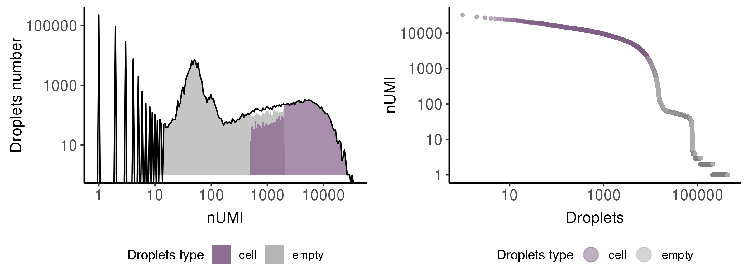
This step is to identify the droplets more likely to include real cells. Generally, Cell Ranger V3 performs this step and shows good performance. In this step, we showed the results by a histogram and a rank plot to present the distribution of total UMI counts (nUMI) in putative cells (purple) and empty droplets (grey)s.

Cell QC

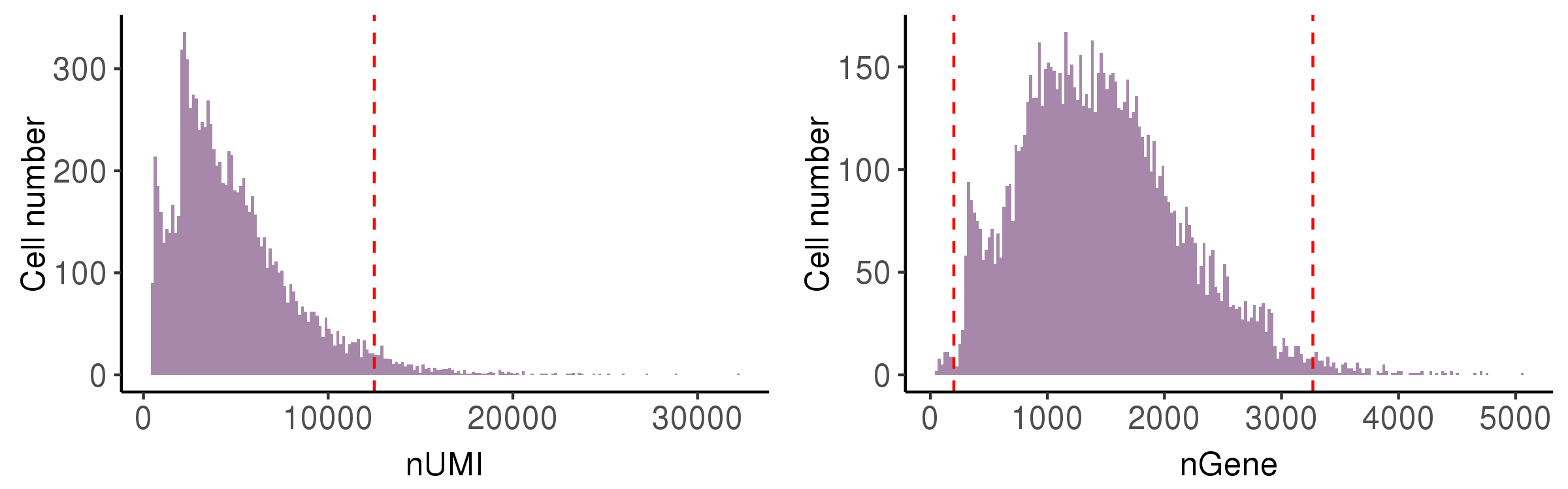
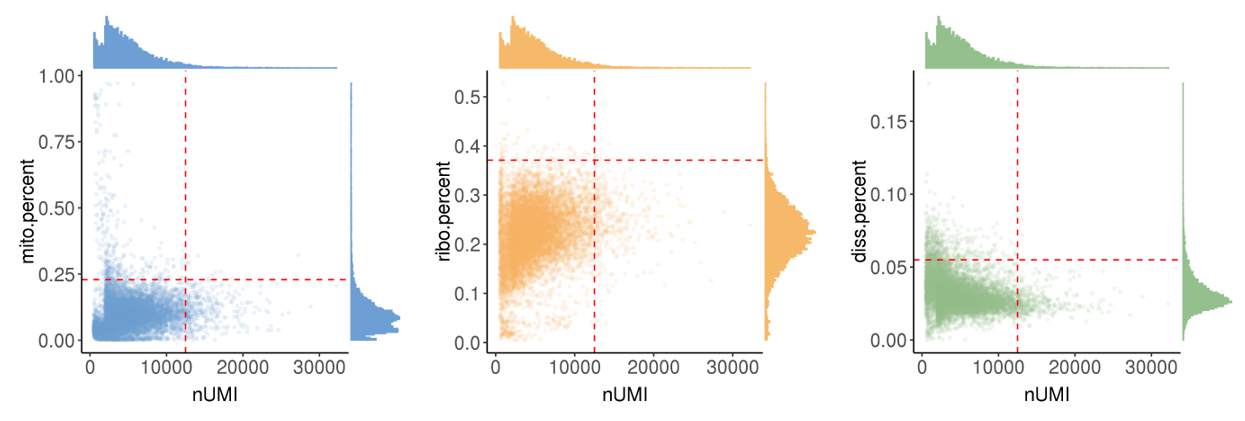
Ideally, one droplet contains one cell in good state and the detected RNA transcripts are all from this cell. However, some abnormal situations may occur, so we calculate following metrics to perform cell quality control (QC).

• nUMI: the number of total UMIs in the droplet. Too small means no cells are captured, and too large means capturing two or more.
• nGene: the number of expressed genes in the droplet. Too small means the loss of transcripts diversity. Too large means containing two or more cells.
• mito.percent: the percentage of UMIs from mitochondrial genes. Too large means the captured cell is necrotic or lysed.
• ribo.percent: the percentage of UMIs from ribosome genes. Too large means the captured cell is necrotic or lysed.
• diss.percent: the percentage of UMIs from dissociation-associated genes. Too large means dissociation process has serious effects on the cell states.

In this step, we showed the distribution of these metrics and provide automatically identified filter thresholds.

The runScAnnotation performs finial cell filter by according to the thresholds recorded in file cell.QC.thres.txt, which is generated by scStatistics. So users can modify the values in the file to adjust the strength of QC. At the same time, the argument bool.filter.cell of function runScAnnotation can control whether to filter cells.

Gene QC

For quality control on genes, we firstly filtered genes which expressed in less than 3 cells. Then, considering that some necrotic or lysed cells may leak their RNA transcripts into the external suspensions, and lead to other droplets being contaminated by these ambient RNA transcripts, we also performed some statistical analyses on the influence of contamination.

In this step, we calculated following three metrics.

• bg.percent : the expression proportion for each gene in background distribution (all droplets with nUMI <= 10)
• prop.median : the median of expression proportions for a gene in each cell.
• detect.rate : the detected (#UMI > 0) rate for a gene in all cells.

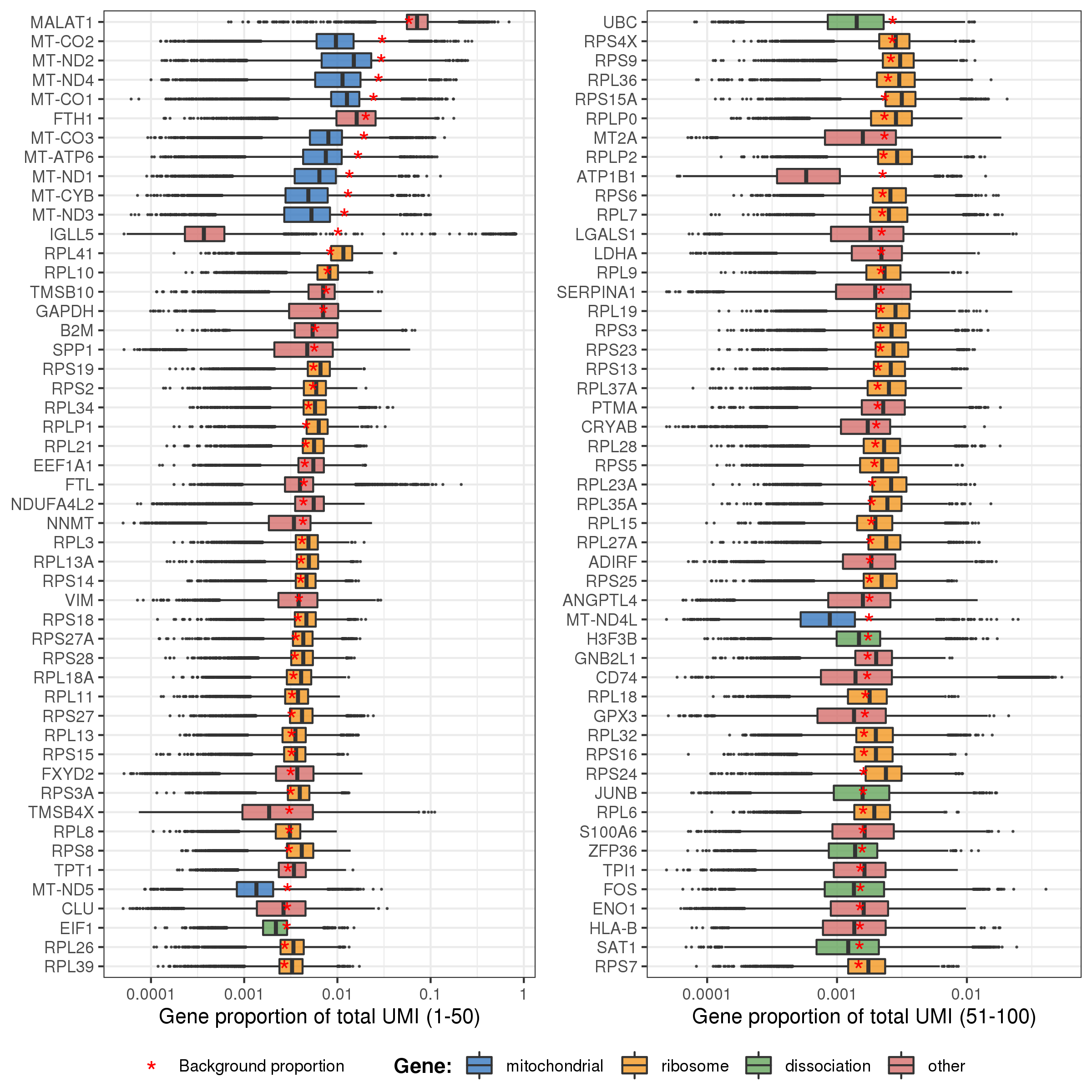
The plot below shows the distributions of gene proportion in cells for the first 100 genes (ordered by their proportion in background bg.percent). And the points (genes) are colored according to whether they belongs to mitochondrial, ribosome, or dissociation associated genes. The red star signs mark the genes’ proportion in background.

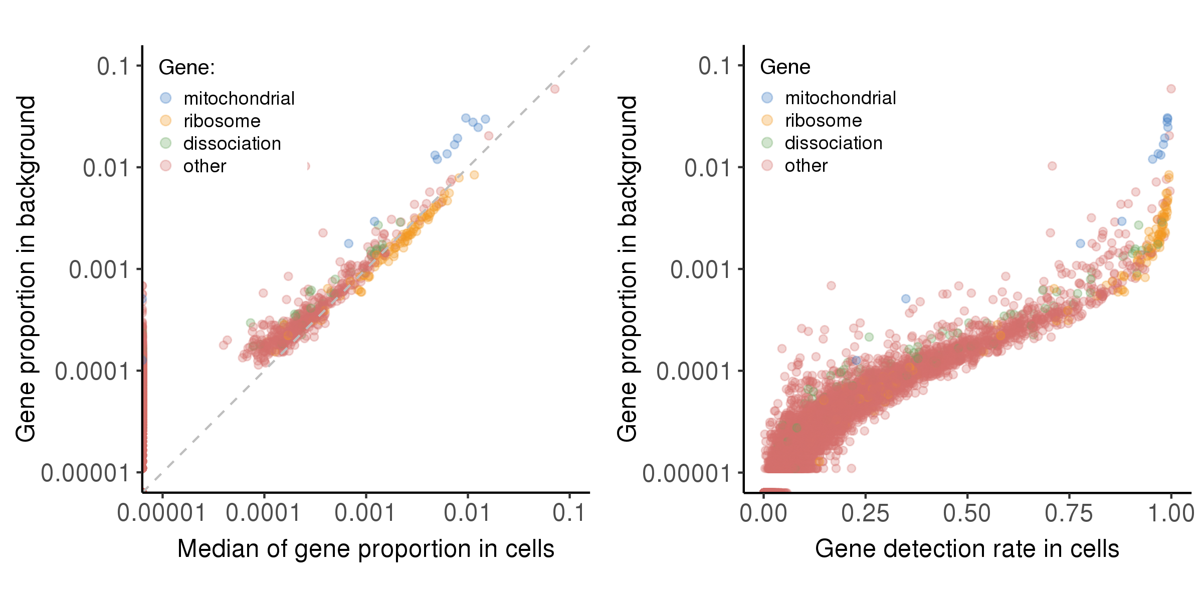
The plot below shows the relationship between bg.percent and prop.median, bg.percent and detect.rate.

The argument bool.filter.cell of function runScAnnotation can control whether to filter genes. If it is TRUE, the argument anno.filter can determine what kind of genes (the default is c("mitochondrial", "ribosome", "dissociation")) are filtered. The argument nCell.min and bgPercent.max can be used to control the gene filter strength of the metrics nCell and bg.percent.

Besides, we also integrated the package SoupX to estimate the contamination fraction of ambient RNAs from lysed cells.

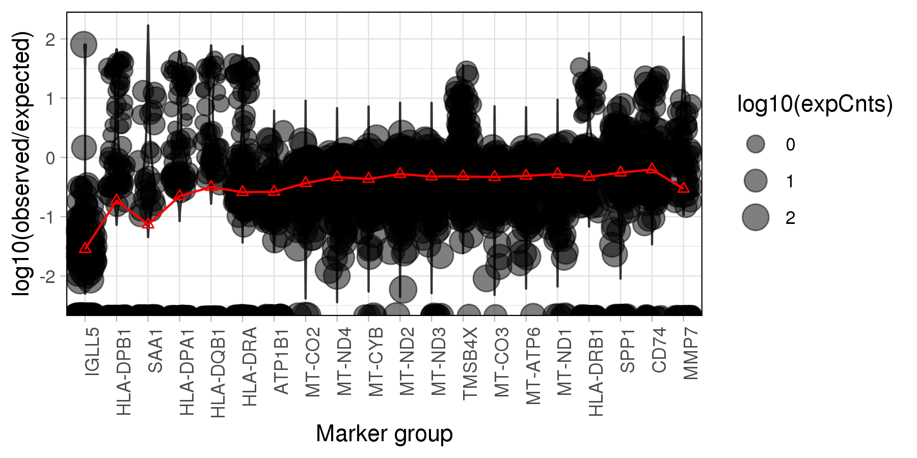
The plot below is generated by SoupX, which visualises the log10 ratios of observed expression counts to expected if the cell is pure background. The read lines marks the estimated contamination fraction using each genes.

Note: The SoupX emphasize that the genes in the plot are heuristic and are just used to help develop biological intuition. It absolutely must not be used to automatically select the top N genes from the list, which may over-estimate the contamination fraction!

By default, we set three default gene sets (immunoglobulin, haemoglobin, and MHC genes) according to the characteristics of cancer microenvironment. Users can input their seleted genes via argument bg.spec.genes to the function runScStatistics. And the argument bool.runSoupx can control whether to perform this step.

Then in scAnnotation module, users can use bool.rmContamination (default is FALSE) to control whether to remove ambient RNA contamination based on SoupX. If it is TRUE, the argument contamination.fraction determines the estimated contamination fraction. If contamination.fraction is NULL, the result of scStatistics will be used.

Basic analyses based on Seurat

The basic analyses of single cell data are mainly performed by Seurat, which included normalization, log-transformation, highly variable genes identification, unwanted variance removing, scaling, centering, dimension reduction (PCA/t-SNE/UMAP), clustering, and differential expression analysis.

In runScAnnotation, following arguments can determine detailed setting of these steps.

• vars.add.meta indicates the variables to be added to Seurat object's meta.data. The default isc("mito.percent", "ribo.percent", "diss.percent").
• vars.to.regress indicates the variables to regress out in Seurat. The default is c("nUMI", "mito.percent", "ribo.percent"). The argument pc.use indicats the number of PCs to use. The default value is 30.
• resolution controls the strength of clustering. The default is 0.8.
• clusterStashName indicates the recorded name of cluster identies. The default is "default".
• show.features indicates the other users interested marker genes to be plotted.
• bool.add.features determines whether to add default marker genes to show.features.
• bool.runDiffExpr determines whether to perform differential expressed analysis.
• n.markers determines the number of differential expressed genes showed in the heatmap. The defalut is 5.

This plot is for highly variable genes.

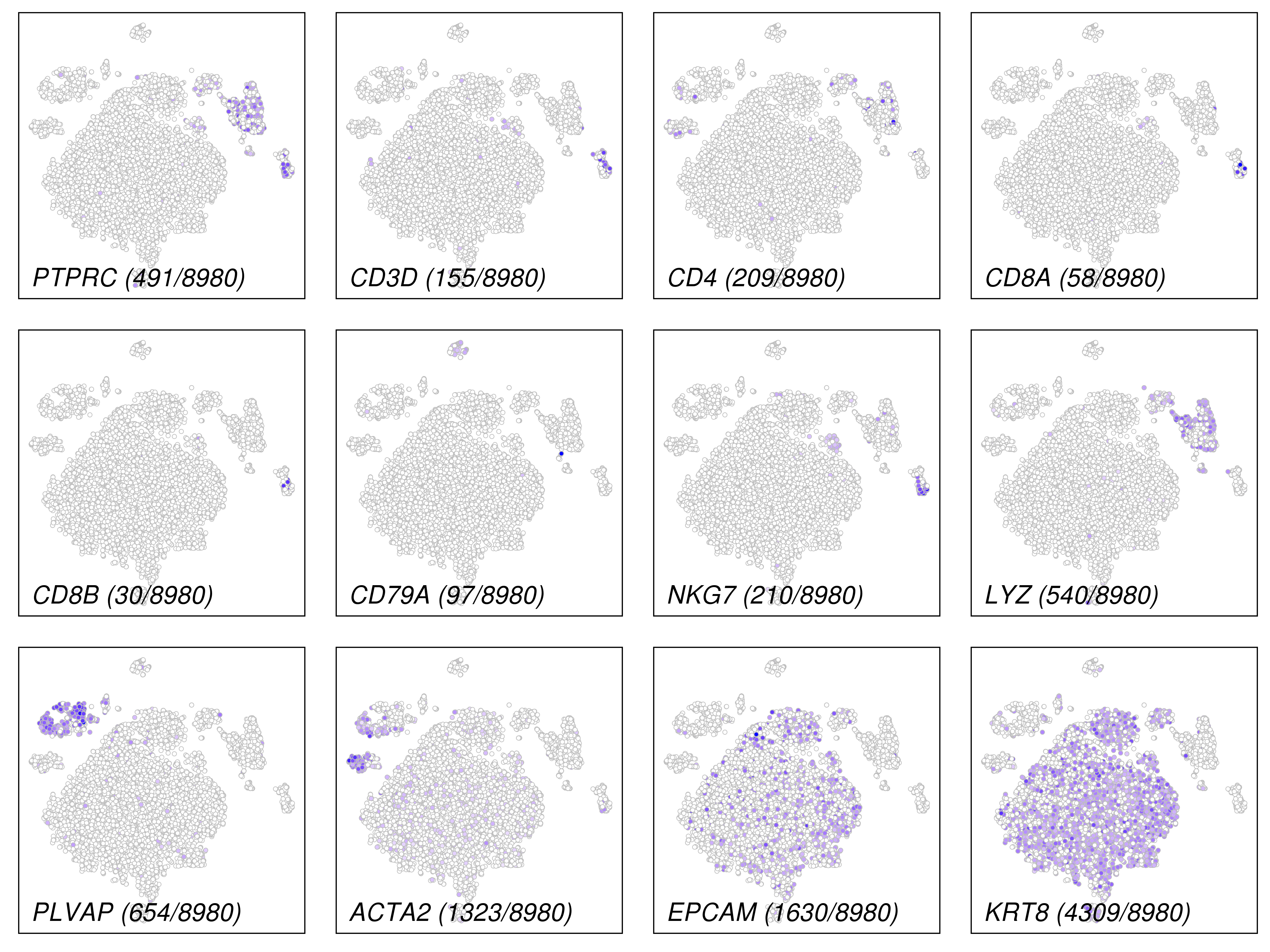
This plot is for common marker genes.

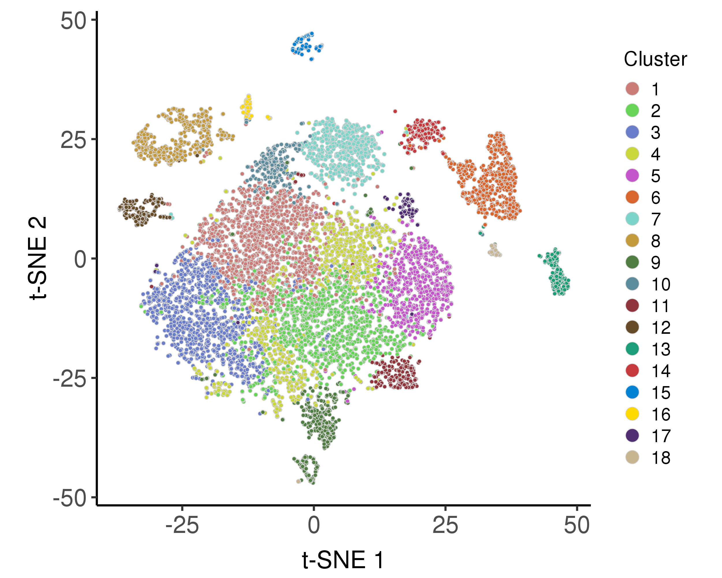
These plots are for clustering on t-SNE and UMAP 2D space.

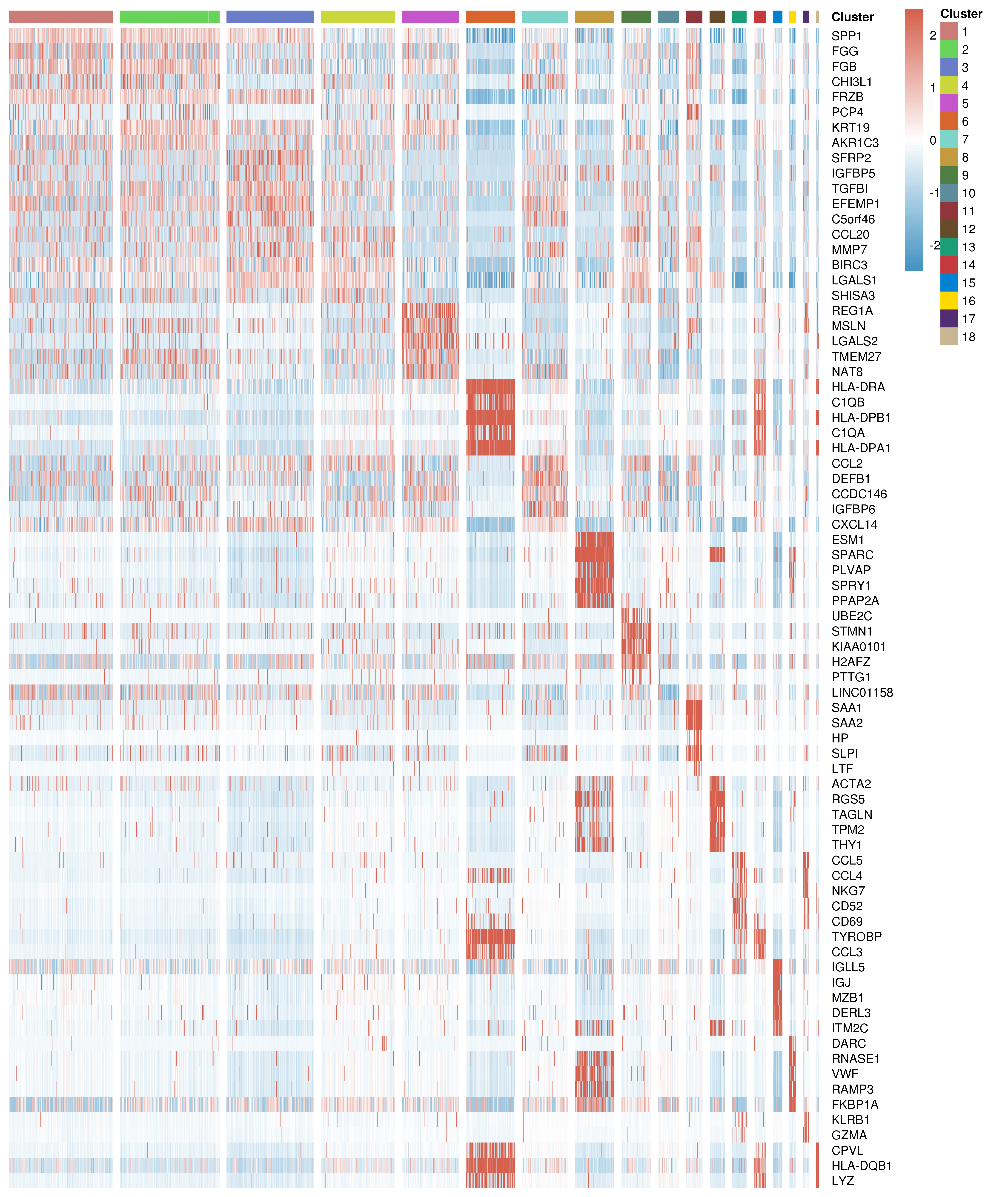
This plot is for differnetial expression analysis.

Doublet scores

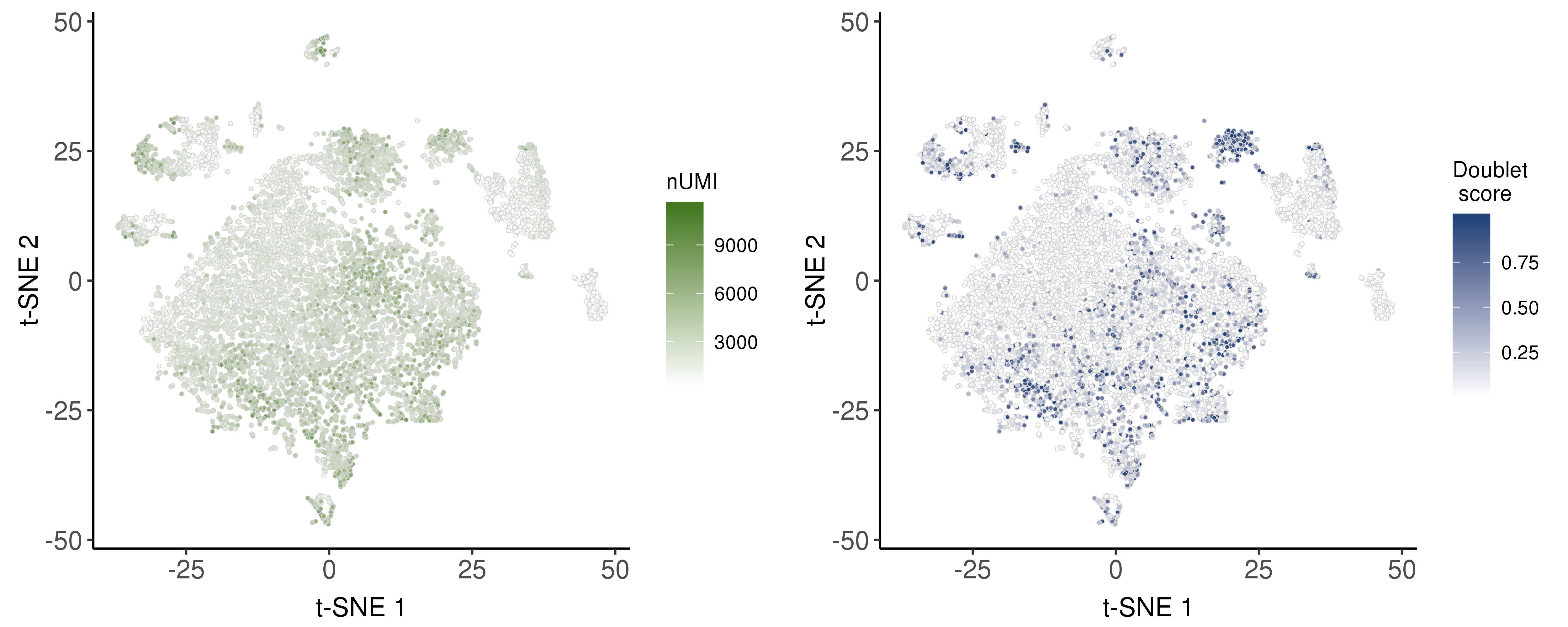
We estimated doublet score based on the package scds.

In runScAnnotation, following arguments can determine detailed setting of this step.

• bool.runDoublet indicates whether to perform this step.
• doublet.method indicates the method to estimate doublet score. The default is "cxds". "cxds"(co-expression based doublet scoring) and "bcds"(binary classification based doublet scoring) are allowed.

Following are the distribution of nUMI and doublet scores.

Cancer micro-environmental cell types annotation

We used one-class logistic regression (OCLR) model to predict common cancer micro-environmental cell types.

In runScAnnotation, following arguments can determine detailed setting of this step.

• bool.runCellClassify indicates whether to predict the usual cell type. The default is TRUE.
• ct.templates indicates OCLR cell type templates used to classification. The default is NULL and eight default templates, including endothelial cells, fibroblasts, and immune cells (CD4+ T cells, CD8+ T cells, B cells, nature killer cells, and myeloid cells) will be used. Users can also train their own templates (the method can be found in next Other personalized settings section.

Following are the distribution of the predicted cell types.

Cell malignancy estimation

The malignancy scores are based on infercnv algorithm.

In runScAnnotation, following arguments can determine detailed setting of this step.

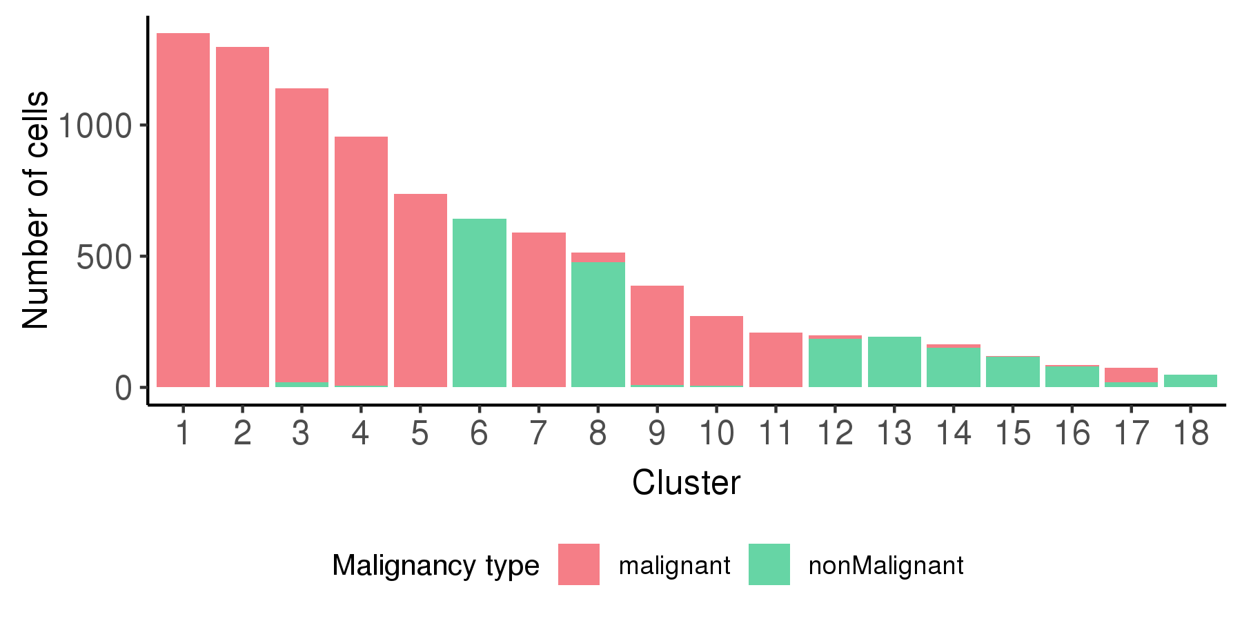
• bool.runMalignancy indicates whether to estimate malignancy.
• cnv.ref.data indicates the expression matrix used as the normal reference. The default is NULL, and an default normal data will be used. User can also input their own reference data by it.
• cnv.referAdjMat indicates the adjacent matrix for the normal reference data. The larger the value, the closer the cell pair is. The default is NULL, and a SNN matrix of the default cnv.ref.data will be used.
• cutoff is a threshold used in the CNV inference.

Following is the distribution of the estimated malignancy scores.

Following is the t-SNE plot colored by malignancy score (left) and type (right).

Following is a bar plot showing the relationship between cell cluster and cell malignancy type.

Intra-tumor heterogeneity analysis

Following intra-tumor phenotypes and signatures heterogeneity analyses are mainly focused tumor cell identified before.

In runScAnnotation, the argument bool.intraTumor indicates whether to use the identified tumor clusters to perform following analyses.

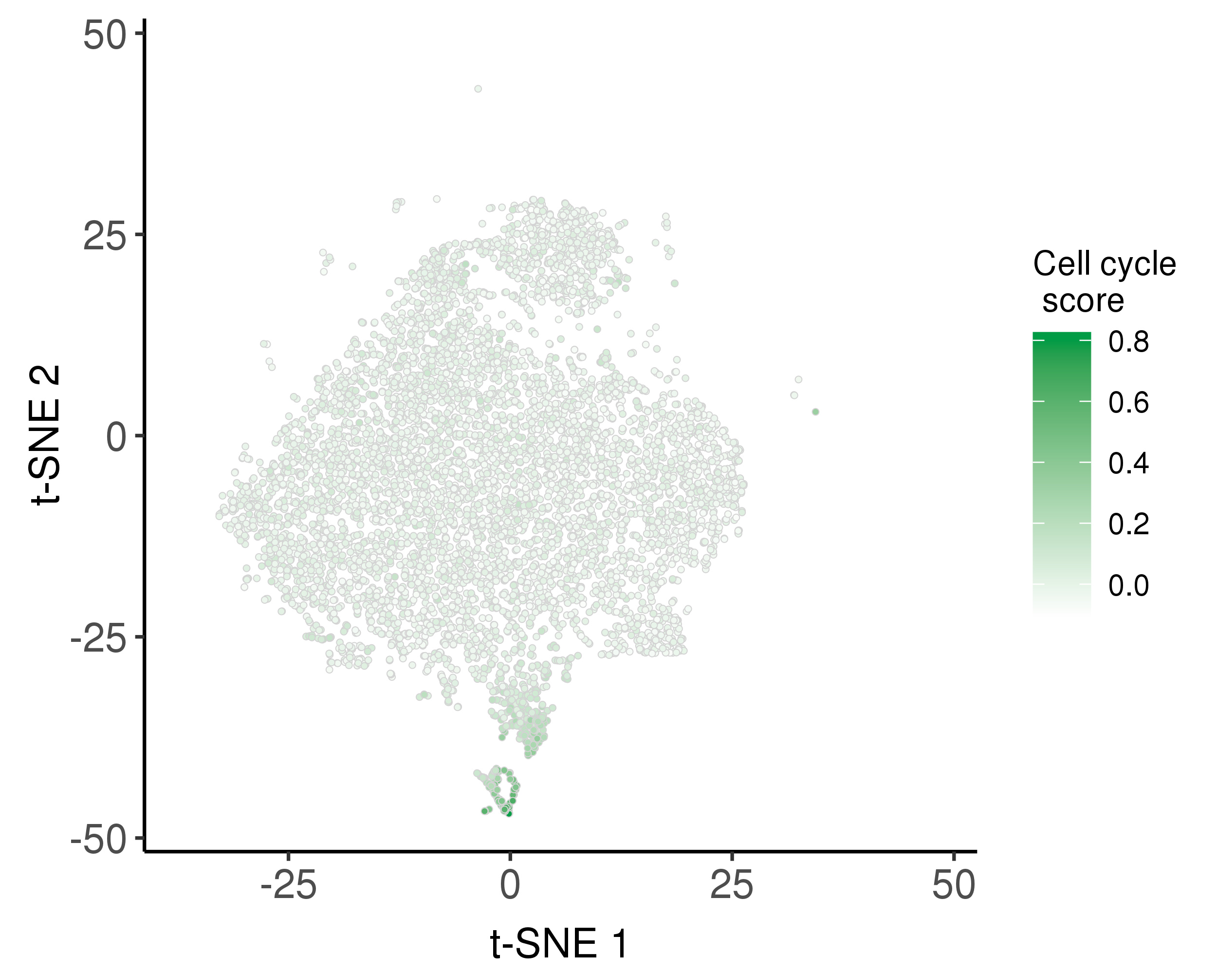
Cell cycle estimation

We used the Seurat AddModuleScore function to calculate the relative average expression of a list of G2/M and S phase markers as cell cycle scores.

In runScAnnotation, following arguments can determine detailed setting of this step.

• bool.runCellCycle indicates whether to estimate cell cycle scores.

Following is the distribution of the estimated cell cycle scores.

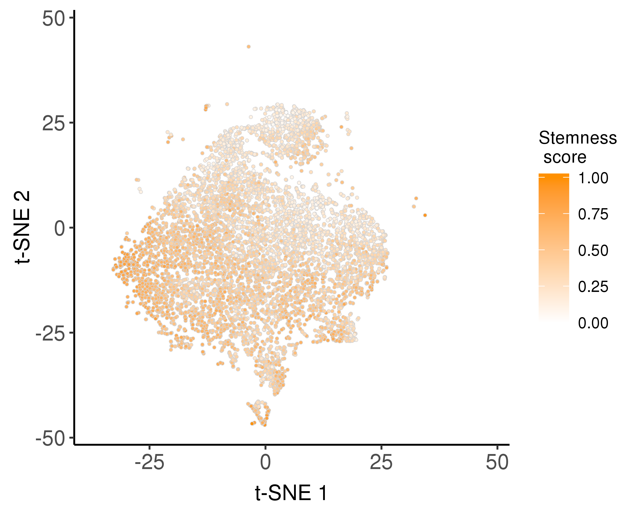
Cell stemness estimation

We trained a stemness signature by OCLR model and use it to estimate stemness scores.

In runScAnnotation, following arguments can determine detailed setting of this step.

• bool.runStemness indicates whether to estimate stemness scores.

Following is the distribution of the estimated stemness scores.

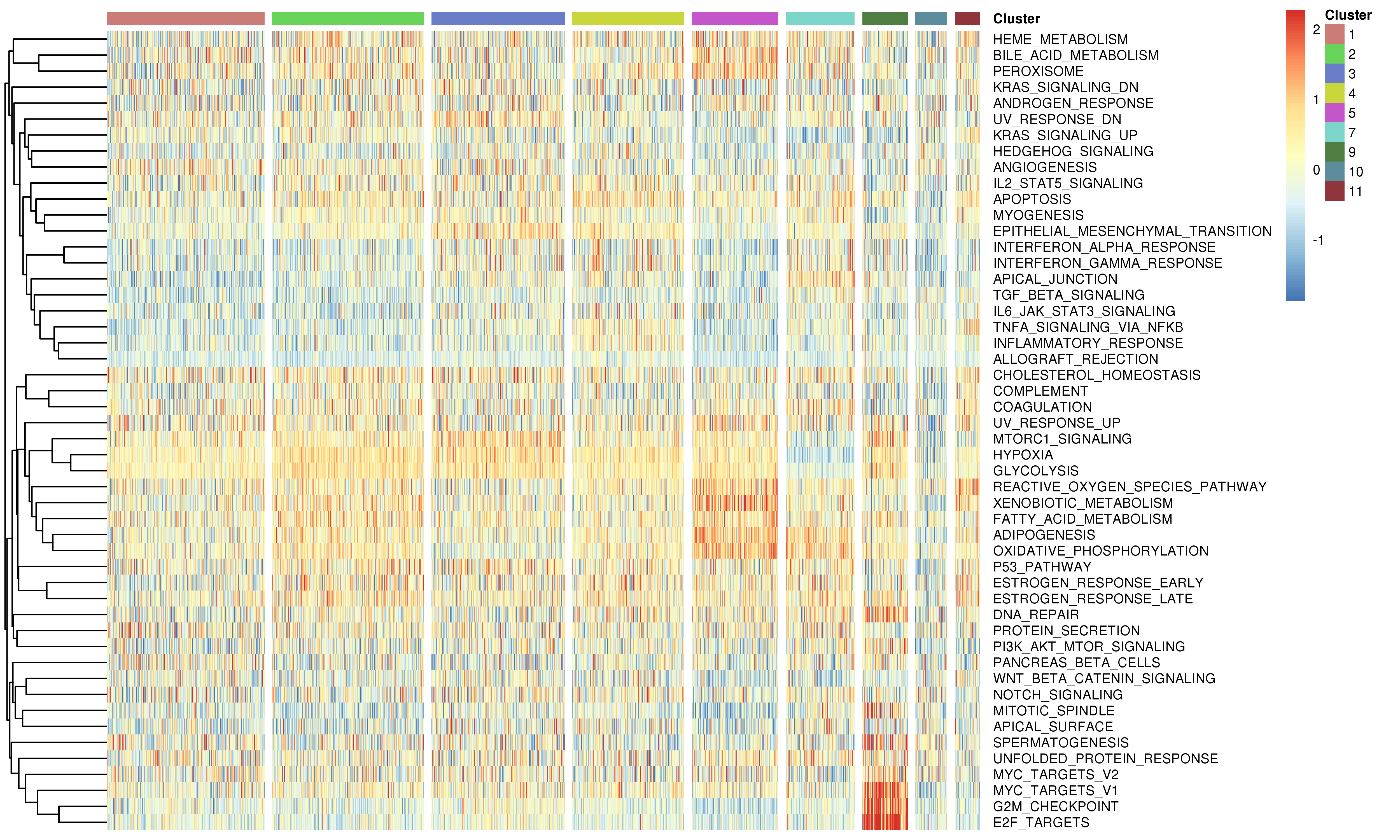
Gene set signature analysis

We provided two approaches to analyze known gene set

For the known gene set signature scores, such as pathways, We provided two approaches. 1.Use gene set variation analysis (GSVA) to estimate variation of the known gene set activities over the cells. 2.Use the relative average expression level across gene sets by using the Seurat AddModuleScore function.

By default, scCancer calculated signature scores of 50 hallmark gene sets from MSigDB and users can also input their own interested gene sets to the function.

In runScAnnotation, following arguments can determine detailed setting of this step.

• bool.runGeneSets indicates whether to estimate stemness scoresestimate gene sets signature scores.
• geneSets indicates the gene sets to be analyzed. It should be list object. The default is NULL and 50 hallmark gene sets from MSigDB will be used.
• geneSet.method indicateds the method to be used in calculate gene set scores. Currently, only average and average are allowed.

Following is the example results of the gene set signature analysis.

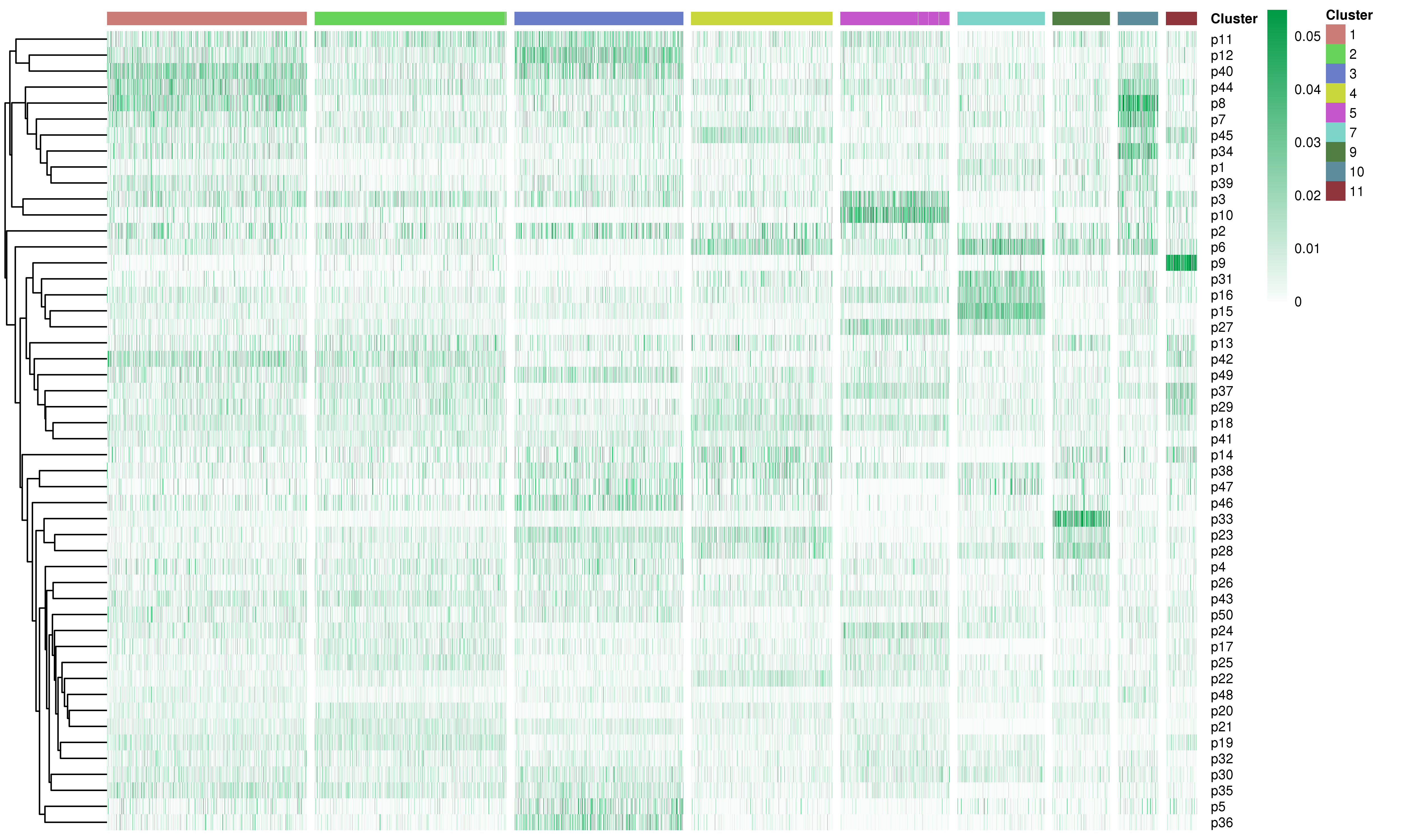
Expression program signatures analysis

We applied non-negative matrix factorization (NMF) to identify potential expression program signatures in unsupervised ways.

In runScAnnotation, following arguments can determine detailed setting of this step.

• bool.runExprProgram indicates whether to run NMF to identify expression programs.
• nmf.rank indicates the decomposition rank used in NMF.

Following is the example results of the expression program signatures analysis.

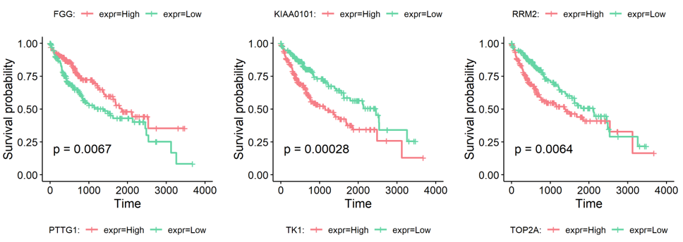
Survival analysis

Based on the type-specific marker genes and gene signatures identified before, we provided an extra function runSurvival to perfrom survival analysis, which read the expression and survival data to plot survival curves and explore the relationship between genes or signatures expression levels and patient prognosis.

In runSurvival, following arguments can determine detailed setting of this step.

• features indicates the names of marker genes or signatures to be analyzed.
• data indicates the data used to perform survival analysis. It should be an expression or signature matrix with gene/signature by patient. The row names are the features' anmes. The columns are patients' labels.
• surv.time indicates the survival time of patients. It should be in accord with the colimns in data.
• surv.event indicates the status indicator of patients. 0=alive, 1=dead. It should be in accord with the colimns in data.
• cut.off indicates the percentage threshold to divide patients into two groups. The default is 0.5, which means the patients are divided by median. Other values, such as 0.4, means the first 40% patients are set "Low" group and the last 40% are set "High" group (the median 20% are discarded).
• savePath indicates the path to save the survival plots of genes/signatures. The default is NULL and the plots will be return without saving.

Following is the example results of survival analysis.

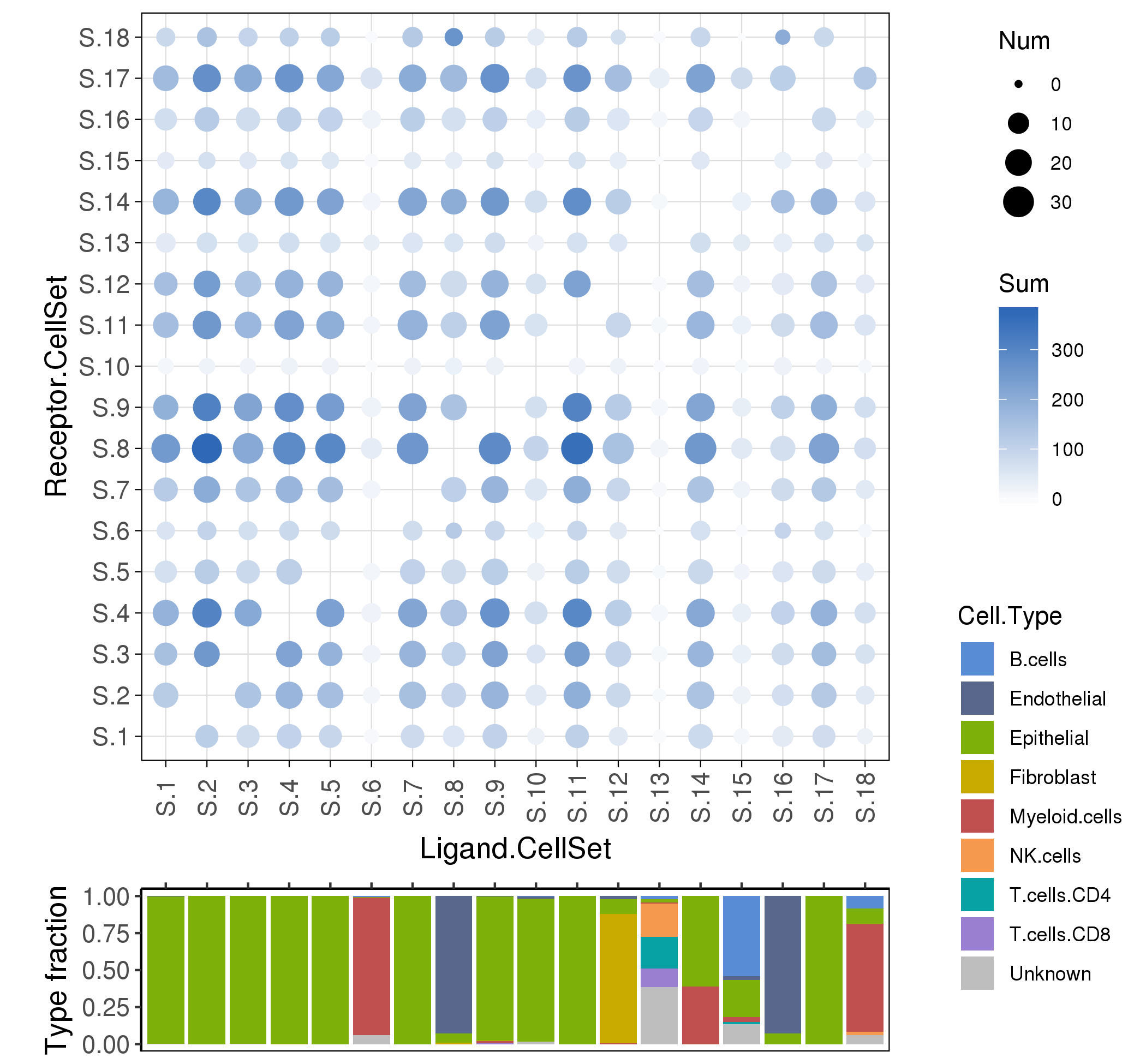
Cell interaction analysis

To analyze the ligand-receptor interactions between the various cell types in cancer micro-environment, we used a ligand-receptor database FANTOM5, and estimate the interaction scores among cell sets (the default is clusters).

Following is the example results of cell interaction analysis.

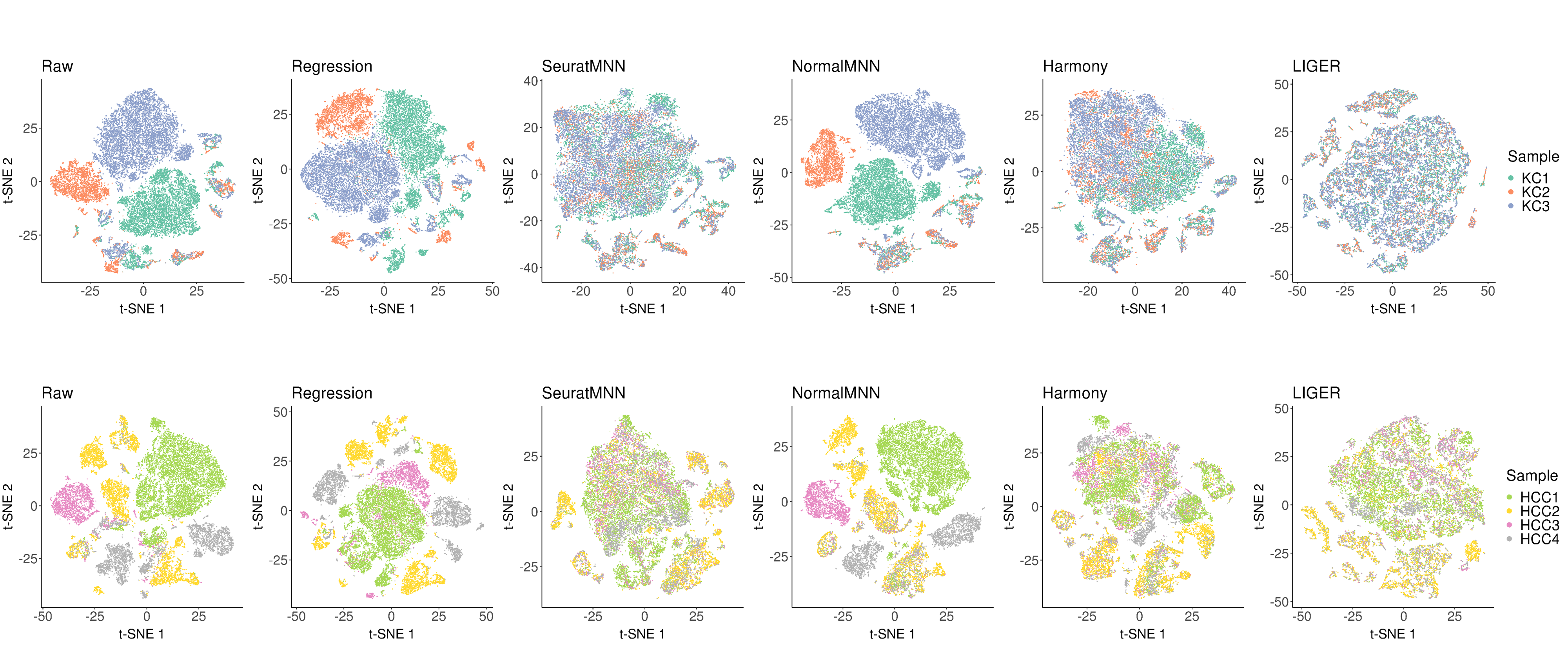
Multi-sample data integration analysis

In scCancer, we provided six approaches to perform multi-sample integration analysis, which covered two of the most basic combination strategies (“Raw”, “Regression”), three best-performing algorithms after systematic evaluation (“SeuratMNN”, “Harmony”, “LIGER”), and a modified MNN version considering the inter-tumor heterogeneity (“NormalMNN”).

In runScCombination, following arguments can determine detailed setting of this step.

• combName indicates the label for the combined samples.
• comb.method indicates the method to combine samples. The default is "NormalMNN". "Harmony", "NormalMNN", "SeuratMNN", "Raw", "Regression" and "LIGER" are optional.
• Other arguments are similar to the single-sample module runScAnnotation.

Following is the example results of the multi-sample data integration analysis.

Other personalized settings

Re-perform cell calling

If the sample data is generated by CR2 and contain "raw_gene_bc_matrices" matrix, the scCancer package can re-perform cell calling using the method EmptyDrop (the name of its R package is DropletUtils). But users need to manually install the DropletUtils and import it in script.

if (!requireNamespace("BiocManager", quietly = TRUE))
    install.packages("BiocManager")
BiocManager::install("DropletUtils")

library(DropletUtils)

Modify cell QC thresholds

After the step scStatistics, a HTML report (report-scStat.html) will be generated, which persents the statistical features of the data from various perspectives (nUMI, nGene, mito.percent, ribo.percent, diss.percent). By identifying outliers from the distribution of these metrics, scCancer adaptively provides some suggested thresholds to filter low-quality cells and records them in the file cell.QC.thres.txt.

Users can modify the values in file cell.QC.thres.txt to make scAnnotation use the updated thresholds to perform cell QC and downstream analyses.

Modify gene QC thresholds

For the step gene QC, the scCancer filters genes according to three aspects of information.

1) Mitochondrial, ribosomal, and dissociation-associated genes. 2) Genes with the number of expressed cells less than argument nCell.min (the default is 3). 3) Genes with the background percentage larger than the argument bgPercent.max (the default is 1, which means unfilter). The bgPercent.max can be decided according to the distribution of background percentage in report-scStat.html.

Users can modify the values of these arguments according to their needs.

Perform ambient RNAs contamination correction

In the scStatistics module, users can pass in the soup (background) specific gene lists by the argument bg.spec.genes or use the default setting:

bg.spec.genes <- list(
    igGenes = c('IGHA1','IGHA2','IGHG1','IGHG2','IGHG3','IGHG4','IGHD','IGHE','IGHM', 'IGLC1','IGLC2','IGLC3','IGLC4','IGLC5','IGLC6','IGLC7', 'IGKC', 'IGLL5', 'IGLL1'),
    HLAGenes = c('HLA-DRA', 'HLA-DRB5', 'HLA-DRB1', 'HLA-DQA1', 'HLA-DQB1', 'HLA-DQB1', 'HLA-DQA2', 'HLA-DQB2', 'HLA-DPA1', 'HLA-DPB1'),
    HBGenes = c("HBB","HBD","HBG1","HBG2", "HBE1","HBZ","HBM","HBA2", "HBA1","HBQ1")
)

Then a contamination fraction will be estimated and saved in file ambientRNA-SoupX.txt.

In the scAnnotation module, if users want to correct the expression data according to the estimated ambient RNAs contamination fraction, they can set the argument bool.rmContamination as TRUE (the default is FALSE), and set the argument contamination.fraction as a number (between 0 and 1) or NULL (NULL means the result of scStatistics will be used).

Set species and genome used for the sample

By default, the arguments species and genome are set as human and hg19. Users can set species as human or mouse, and set genome as hg19, hg38, or mm10, respectively.

Analyze PDX samples

Patient-drived tumor xenograft (PDX) samples contain both human and mouse cells generally. In order to deal with these human-mouse-mixed data, users can explicitly set the arguments hg.mm.mix, species, genome, hg.mm.thres, and mix.anno of the relevant functions. More details for the meaning of these arguments can be found by using command help().

Use "UMAP" coordinates to present analyses results

By default, we use both t-SNE and UMAP to obtain low-dimension coordiantes, and the clustering results are presented using both of them. For other analyses, we use t-SNE 2D coordinates by default. Users can also set the argument coor.names as c("UMAP_1", "UMAP_2") to view the results under UMAP coordinates.

Note: If users haven't installed UMAP, they can do so via ```{python eval=FALSE} reticulate::py_install(packages = 'umap-learn')

## Analyze multi-modal data
For the multi-modal data, which have both gene expression and antibody capture results, `scCancer` is also compatible. Users don't need to perform special setting, and `scCancer` will extract the expression data automatically and run downstream analyses.


## Train new cell type templates
If users' samples have other cell types to classify, they can train the new templates and pass in the argument `ct.templates`. To train the new templates, following cods can be referred:

```r
library(gelnet)

train.data <- list("type1" = expr.data1, "type2" = expr.data2)
ct.templates <- lapply(names(train.data), FUN = function(x){
    result <- gelnet(t(train.data[[x]]), NULL, 0, 1)
    return(result$w[result$w != 0])
})

Session Information

Here is the output of sessionInfo() on the system.

R version 3.6.1 (2019-07-05)
Platform: x86_64-pc-linux-gnu (64-bit)
Running under: CentOS Linux 7 (Core)

Matrix products: default

locale:
 [1] LC_CTYPE=en_US.UTF-8       LC_NUMERIC=C
 [3] LC_TIME=en_US.UTF-8        LC_COLLATE=en_US.UTF-8
 [5] LC_MONETARY=en_US.UTF-8    LC_MESSAGES=en_US.UTF-8
 [7] LC_PAPER=en_US.UTF-8       LC_NAME=C
 [9] LC_ADDRESS=C               LC_TELEPHONE=C
[11] LC_MEASUREMENT=en_US.UTF-8 LC_IDENTIFICATION=C

attached base packages:
[1] stats     graphics  grDevices utils     datasets  methods   base

other attached packages:
[1] scCancer_2.0.0

loaded via a namespace (and not attached):
  [1] sn_1.5-4                    plyr_1.8.5
  [3] igraph_1.2.4.2              lazyeval_0.2.2
  [5] GSEABase_1.48.0             splines_3.6.1
  [7] BiocParallel_1.20.1         listenv_0.8.0
  [9] GenomeInfoDb_1.22.0         ggplot2_3.2.1
 [11] TH.data_1.0-10              digest_0.6.23
 [13] htmltools_0.4.0             gdata_2.18.0
 [15] magrittr_1.5                memoise_1.1.0
 [17] cluster_2.1.0               ROCR_1.0-7
 [19] globals_0.12.5              annotate_1.64.0
 [21] matrixStats_0.55.0          RcppParallel_4.4.4
 [23] R.utils_2.9.2               sandwich_2.5-1
 [25] colorspace_1.4-1            blob_1.2.0
 [27] rappdirs_0.3.1              ggrepel_0.8.1
 [29] xfun_0.11                   dplyr_0.8.3
 [31] crayon_1.3.4                RCurl_1.95-4.12
 [33] jsonlite_1.6                graph_1.64.0
 [35] survival_3.1-8              zoo_1.8-7
 [37] ape_5.3                     glue_1.3.1
 [39] gtable_0.3.0                zlibbioc_1.32.0
 [41] XVector_0.26.0              leiden_0.3.2
 [43] DelayedArray_0.12.1         future.apply_1.4.0
 [45] SingleCellExperiment_1.8.0  BiocGenerics_0.32.0
 [47] scales_1.1.0                pheatmap_1.0.12
 [49] mvtnorm_1.0-12              DBI_1.1.0
 [51] bibtex_0.4.2.2              miniUI_0.1.1.1
 [53] Rcpp_1.0.3                  metap_1.3
 [55] plotrix_3.7-7               viridisLite_0.3.0
 [57] xtable_1.8-4                reticulate_1.14
 [59] bit_1.1-14                  rsvd_1.0.2
 [61] SDMTools_1.1-221.2          stats4_3.6.1
 [63] tsne_0.1-3                  GSVA_1.34.0
 [65] NNLM_0.4.3                  scds_1.2.0
 [67] htmlwidgets_1.5.1           httr_1.4.1
 [69] gplots_3.0.1.2              RColorBrewer_1.1-2
 [71] TFisher_0.2.0               Seurat_3.1.2
 [73] ica_1.0-2                   pkgconfig_2.0.3
 [75] XML_3.98-1.20               R.methodsS3_1.7.1
 [77] uwot_0.1.5                  tidyselect_1.0.0
 [79] rlang_0.4.4                 reshape2_1.4.3
 [81] later_1.0.0                 AnnotationDbi_1.48.0
 [83] munsell_0.5.0               tools_3.6.1
 [85] xgboost_0.90.0.2            RSQLite_2.1.5
 [87] ggridges_0.5.2              stringr_1.4.0
 [89] fastmap_1.0.1               npsurv_0.4-0
 [91] knitr_1.26                  bit64_0.9-7
 [93] fitdistrplus_1.0-14         caTools_1.18.0
 [95] purrr_0.3.3                 RANN_2.6.1
 [97] pbapply_1.4-2               future_1.16.0
 [99] nlme_3.1-143                mime_0.8
[101] R.oo_1.23.0                 ggExtra_0.9
[103] compiler_3.6.1              shinythemes_1.1.2
[105] plotly_4.9.1                png_0.1-7
[107] lsei_1.2-0                  tibble_2.1.3
[109] geneplotter_1.64.0          stringi_1.4.5
[111] lattice_0.20-38             Matrix_1.2-18
[113] markdown_1.1                multtest_2.42.0
[115] vctrs_0.2.2                 mutoss_0.1-12
[117] pillar_1.4.3                lifecycle_0.1.0
[119] Rdpack_0.11-1               lmtest_0.9-37
[121] RcppAnnoy_0.0.14            data.table_1.12.8
[123] cowplot_1.0.0               bitops_1.0-6
[125] irlba_2.3.3                 gbRd_0.4-11
[127] GenomicRanges_1.38.0        httpuv_1.5.2
[129] R6_2.4.1                    promises_1.1.0
[131] KernSmooth_2.23-16          gridExtra_2.3
[133] IRanges_2.20.1              codetools_0.2-16
[135] MASS_7.3-51.5               gtools_3.8.1
[137] assertthat_0.2.1            SummarizedExperiment_1.16.1
[139] sctransform_0.2.1           mnormt_1.5-5
[141] multcomp_1.4-12             S4Vectors_0.24.1
[143] GenomeInfoDbData_1.2.2      parallel_3.6.1
[145] SoupX_1.0.1                 grid_3.6.1
[147] tidyr_1.0.2                 Rtsne_0.15
[149] pROC_1.15.3                 numDeriv_2016.8-1.1
[151] Biobase_2.46.0              shiny_1.4.0

wguo-research/scCancer documentation built on May 26, 2024, 9:12 p.m.